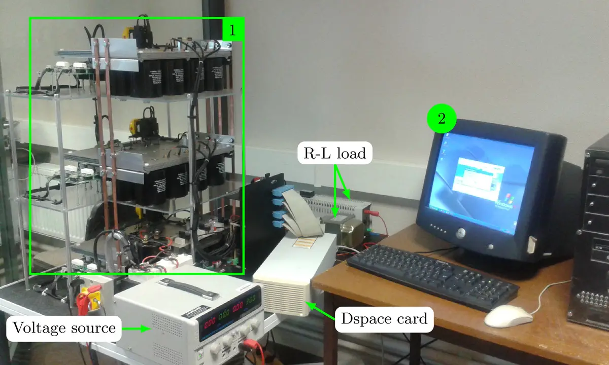
Let's get into the detail!
Step 1: Include an image in TikZ
In LaTeX, we use \includegraphics command to add an image which requires loading the package graphicx. In TikZ, we will use the same command inside a node. Here is an illustrative example:
\documentclass{standalone}

\usepackage{tikz}

\begin{document}

\begin{tikzpicture}

	\node (image) at (0,0) {
		\includegraphics[width=\textwidth]{example-image}
	};

\end{tikzpicture}

\end{document}
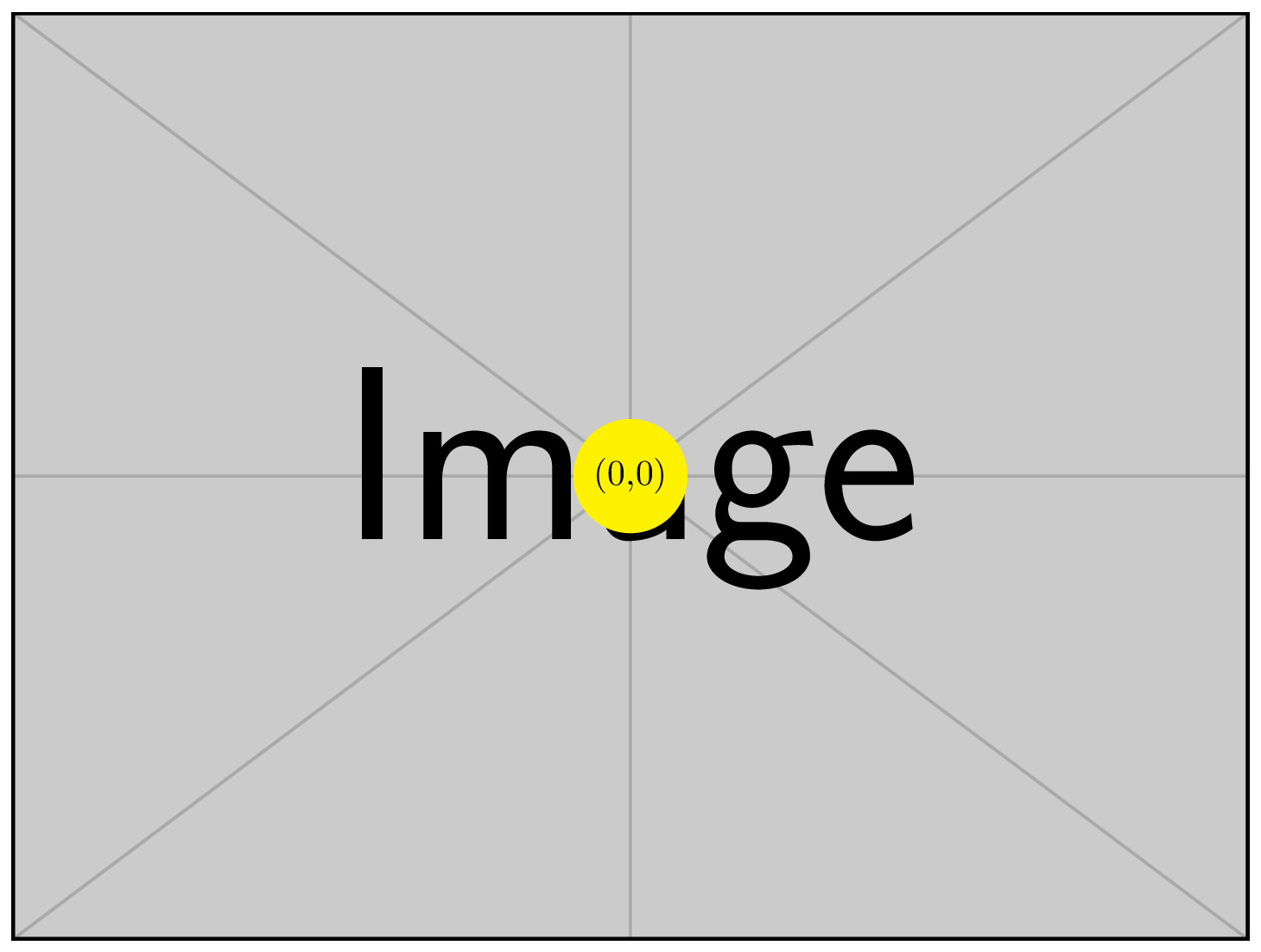
Image added inside a node in TikZ
Comments:
- We loaded the TikZ package using \usepackage{tikz}. It should be noted that there is no need to load graphicx package as it is already loaded by TikZ.
- We created a node at the point with coordinates (0,0) and we named it (image).
- The image, with name (image), is added using \includegraphics command with a width equal to the text width of the document. I invite you to check the set of images that can be used for creating a minimal working example (MWE).
a. Positioning Nodes using Anchors
For easier positioning, It is better to put the origin at the bottom left corner of the image. This can be achieved by modifying the anchor of the node as follows:
\documentclass{standalone}

\usepackage{tikz}

\begin{document}

\begin{tikzpicture}

\node[anchor=south west] (image) at (0,0) {
	\includegraphics[width=\textwidth]{example-image}
};

\end{tikzpicture}

\end{document}
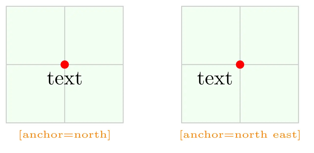
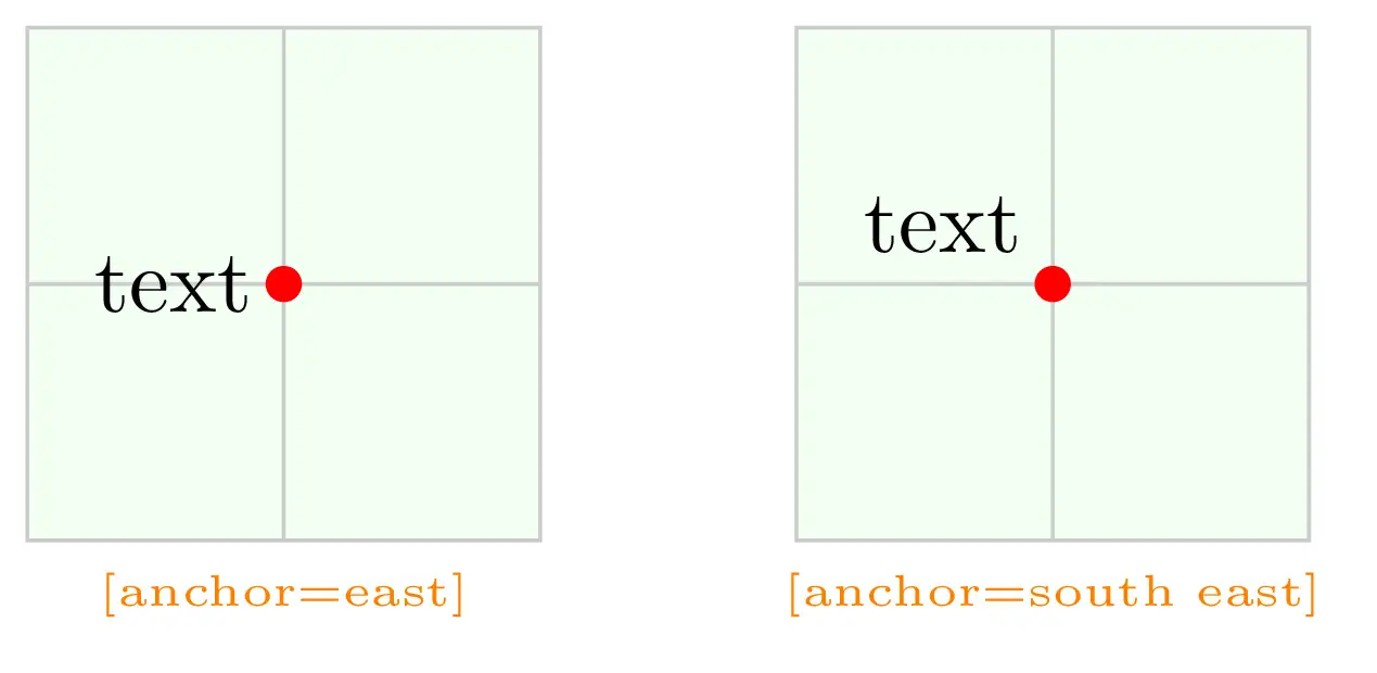
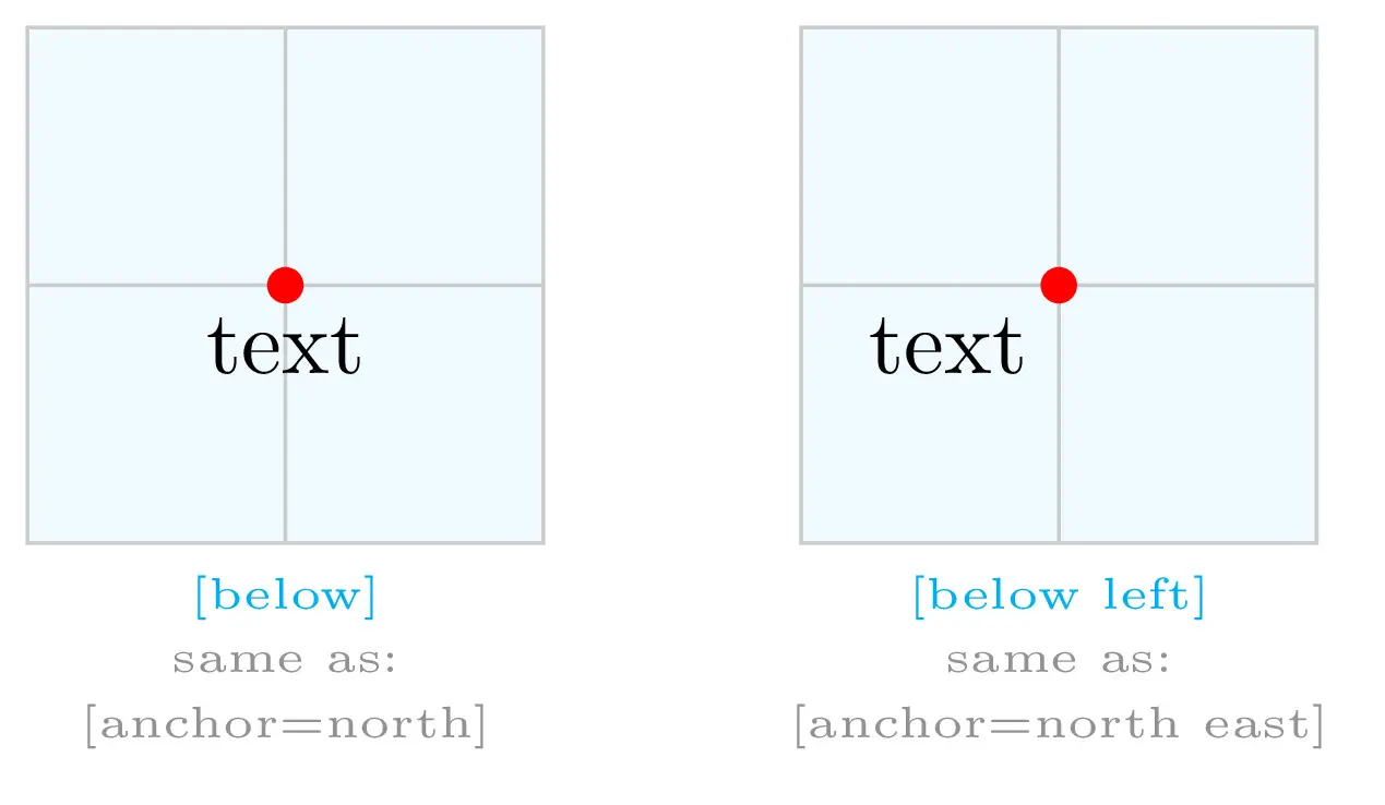
We simply added the option anchor=south west to the \node command. Here is a list of different cases. We used the word text instead of an image without loss of generality.
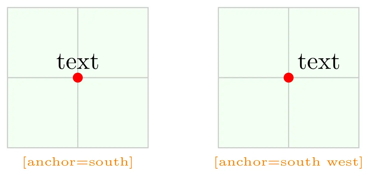
Positioning nodes using anchor mechanism 1
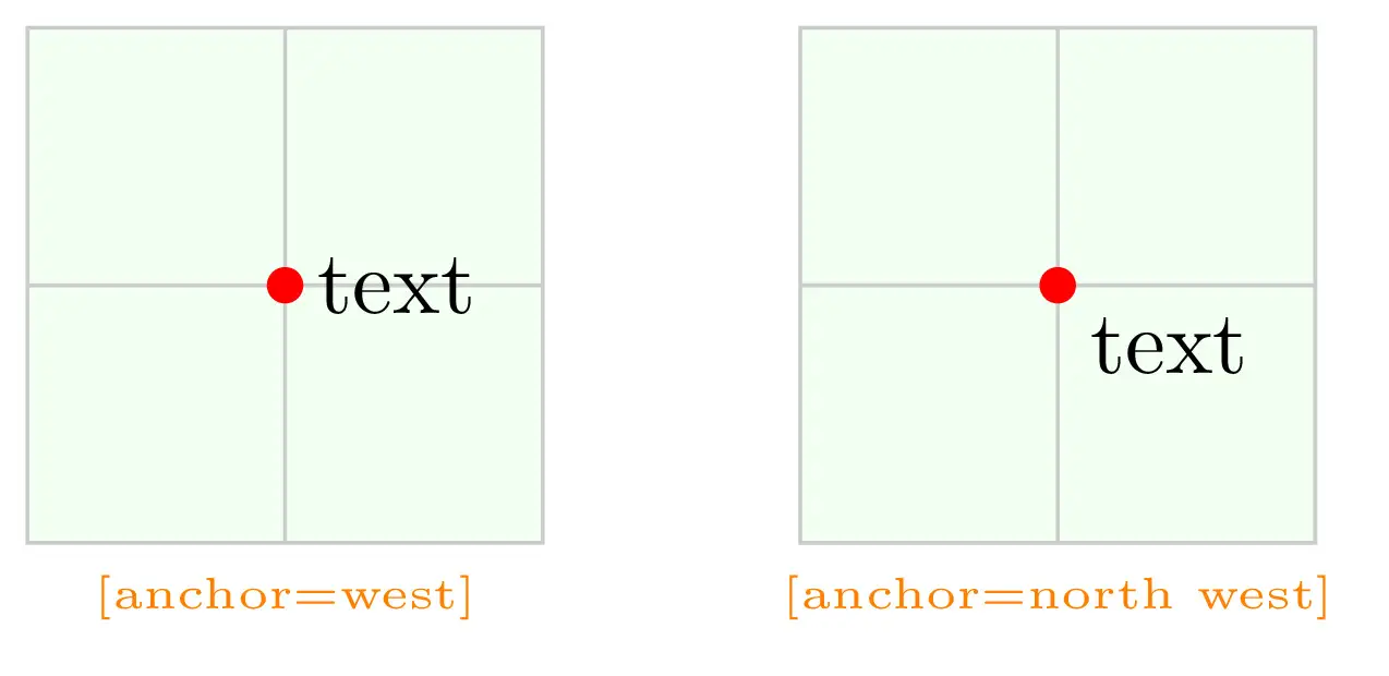
Positioning nodes using anchor mechanism 2
Positioning nodes using anchor mechanism 3
Positioning nodes using anchor mechanism 4
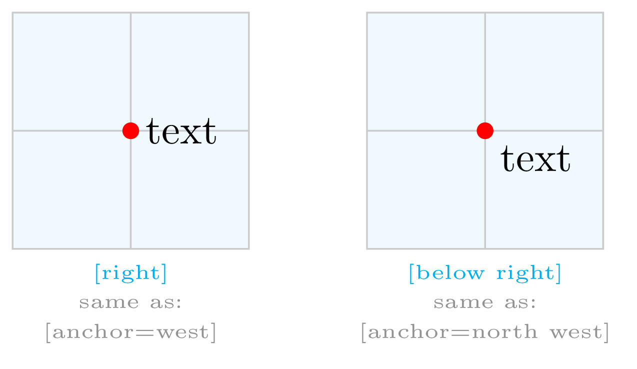
To be honest, I prefer to use the basic placement options instead of the anchoring mechanism as It provides the location of the text (or the image) with respect to the coordinates. Here is a list that compares both positioning approaches and for more details, check the manual "section: Positioning Nodes".
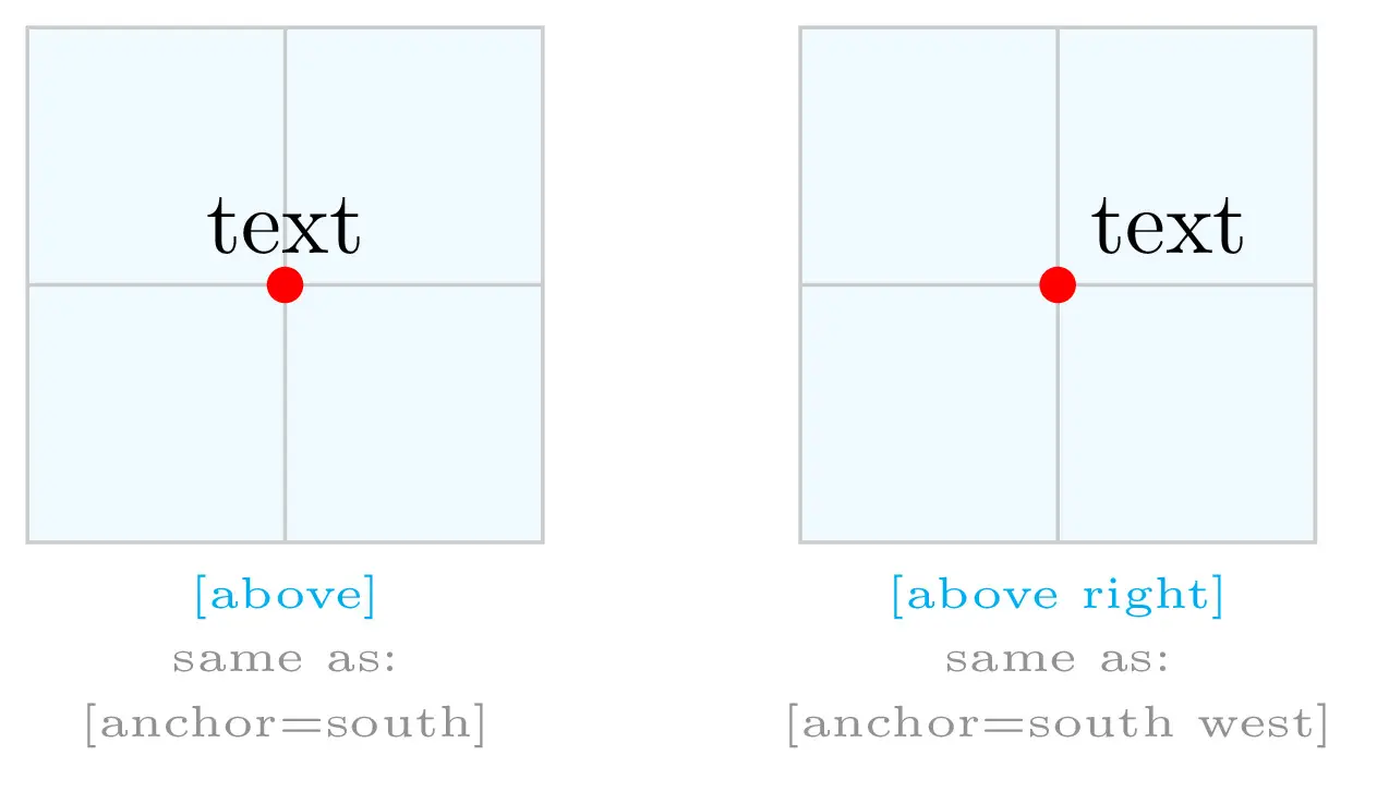
Basic placement VS anchor mechanism 1
Basic placement VS anchor mechanism 2
Basic placement VS anchor mechanism 3
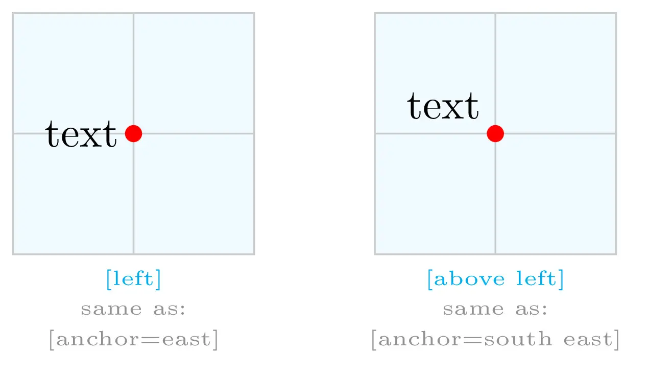
Basic placement VS anchor mechanism 4
Using the basic placement option, we put the image above and right of the (0,0). Here is the corresponding code in this case:
\documentclass{standalone}

\usepackage{tikz}

\begin{document}

\begin{tikzpicture}

\node[above right] (image) at (0,0) {
	\includegraphics[width=\textwidth]{example-image}
};

\end{tikzpicture}

\end{document}
It should be noted that above right is different than above,right. In the latter, the option right will be used as it is the last option for positioning.
b. Remove Inner Separation
You may remarked in the previous illustration a small white margin induced by the node command. It can be controlled by adding the option inner separation=value to the \node command. This allows us to precisely put the origin at the bottom left corner of the image.
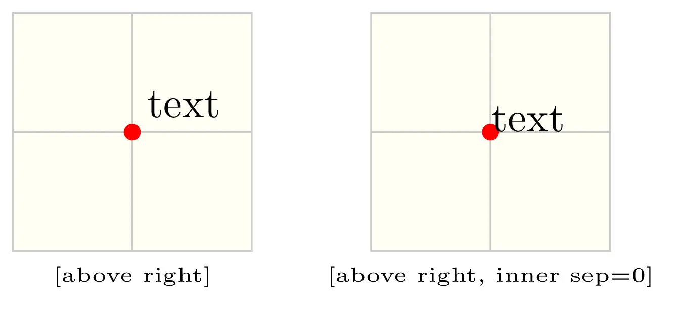
Setting the inner separation in TikZ
Here is the final code of step 1 (include the image in a node):
\documentclass{standalone}

\usepackage{tikz}

\begin{document}

\begin{tikzpicture}

\node[above right, inner sep=0] (image) at (0,0) {
	\includegraphics[width=\textwidth]{example-image}
};

\end{tikzpicture}

\end{document}
Step 2: Image with axes
Now, we need to add axes with a grid in order to be able to put labels at specific positions in the image. These positions are relative to the image size which allows us to resize our illustration without any issues (arrows and shapes will also be resized automatically).
This can be done using a scope environment as below:
 \documentclass{standalone}

\usepackage{tikz}
\usetikzlibrary{calc}

\begin{document}

\begin{tikzpicture}

% Include the image in a node
\node [
	above right,
	inner sep=0] (image) at (0,0) {\includegraphics[width=\textwidth]{example-image}};

% Create scope with normalized axes
\begin{scope}[
x={($0.1*(image.south east)$)},
y={($0.1*(image.north west)$)}]

% Grid
	\draw[lightgray,step=1] (image.south west) grid (image.north east);
\end{scope}

\end{tikzpicture}

\end{document}
where we get an image with 10x10 grid:
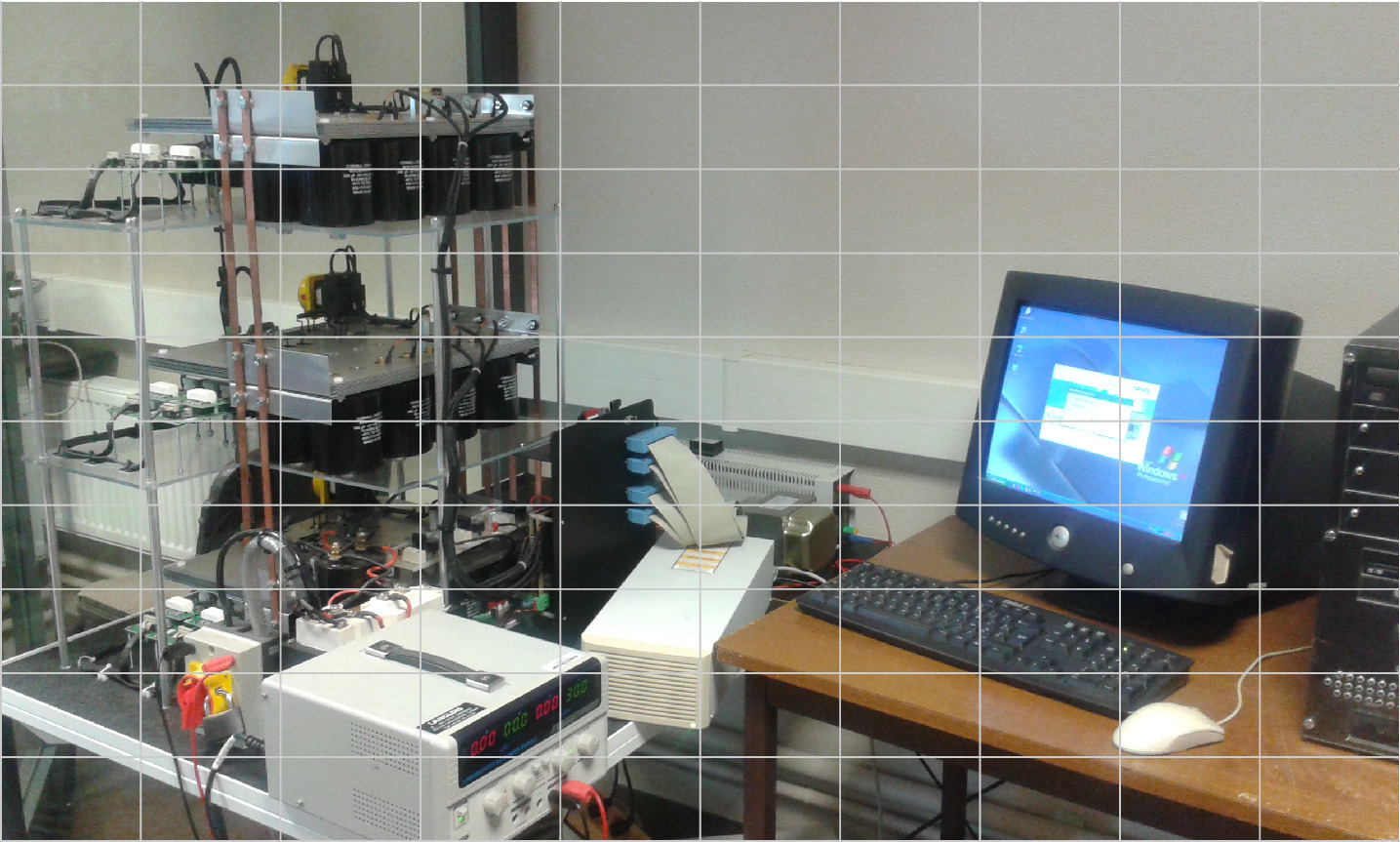
Comments:
- In the scope, we specified x=<value> and y=<value> for axes units. The x-axis unit is chosen one tenth the image width. The y-axis unit is chosen one tenth the image height.
- The image width and height are obtained from (image.south east) and (image.north west), respectively.
- For coordinate calculations, we loaded the TikZ library calc. It allows us to choose the one tenth of the image size as units for the axes.
- We created a grid using the command grid between the image corners: (image.south west) and (image.north east).
- Grid lines are chosen with a light gray color and a step of 1 (normalized unit). For a more precision, you can modify the step to a smaller value.
Let's add labels and as it is a repetitive thing we will use a for loop (read this post to learn how to use foreach loop).
Here is the final code of step 2 (add axes and labels):
 \documentclass{standalone}

\usepackage{tikz}
\usetikzlibrary{calc}

\begin{document}

\begin{tikzpicture}

% Include the image in a node
\node [
	above right,
	inner sep=0] (image) at (0,0) {\includegraphics[width=\textwidth]{example-image}};

% Create scope with normalized axes
\begin{scope}[
	x={($0.1*(image.south east)$)},
	y={($0.1*(image.north west)$)}]

% Grid
	\draw[lightgray,step=1] (image.south west) grid (image.north east);

% Axes' labels
	\foreach \x in {0,1,...,10} { \node [below] at (\x,0) {\x}; }
	\foreach \y in {0,1,...,10} { \node [left] at (0,\y) {\y};}

\end{scope}

\end{tikzpicture}

\end{document}
and the corresponding image:
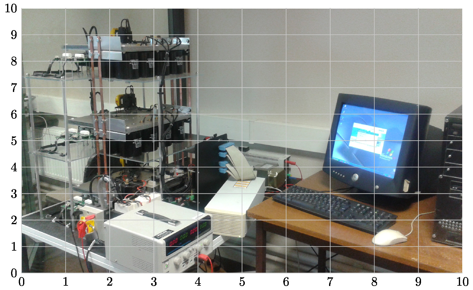
Comments:
- We used two \foreach loops, one for the x-axis labels and one for the y-axis labels. The loop counter varies from 0 to 10 with an increment equal to 1.
- The loop counter (\x and \y) is used for coordinates and for printing labels.
- At each value of the loop counter of the x-axis, we add a node below the coordinates by providing the option below, check above the basic placement options.
- The same for the y-axis, we use the option left to print labels on the left of the y-axis.
Labels, circles and arrows will be added inside the scope in question, which is the aim of the next section!
Step 3: Add labels, circles and arrows
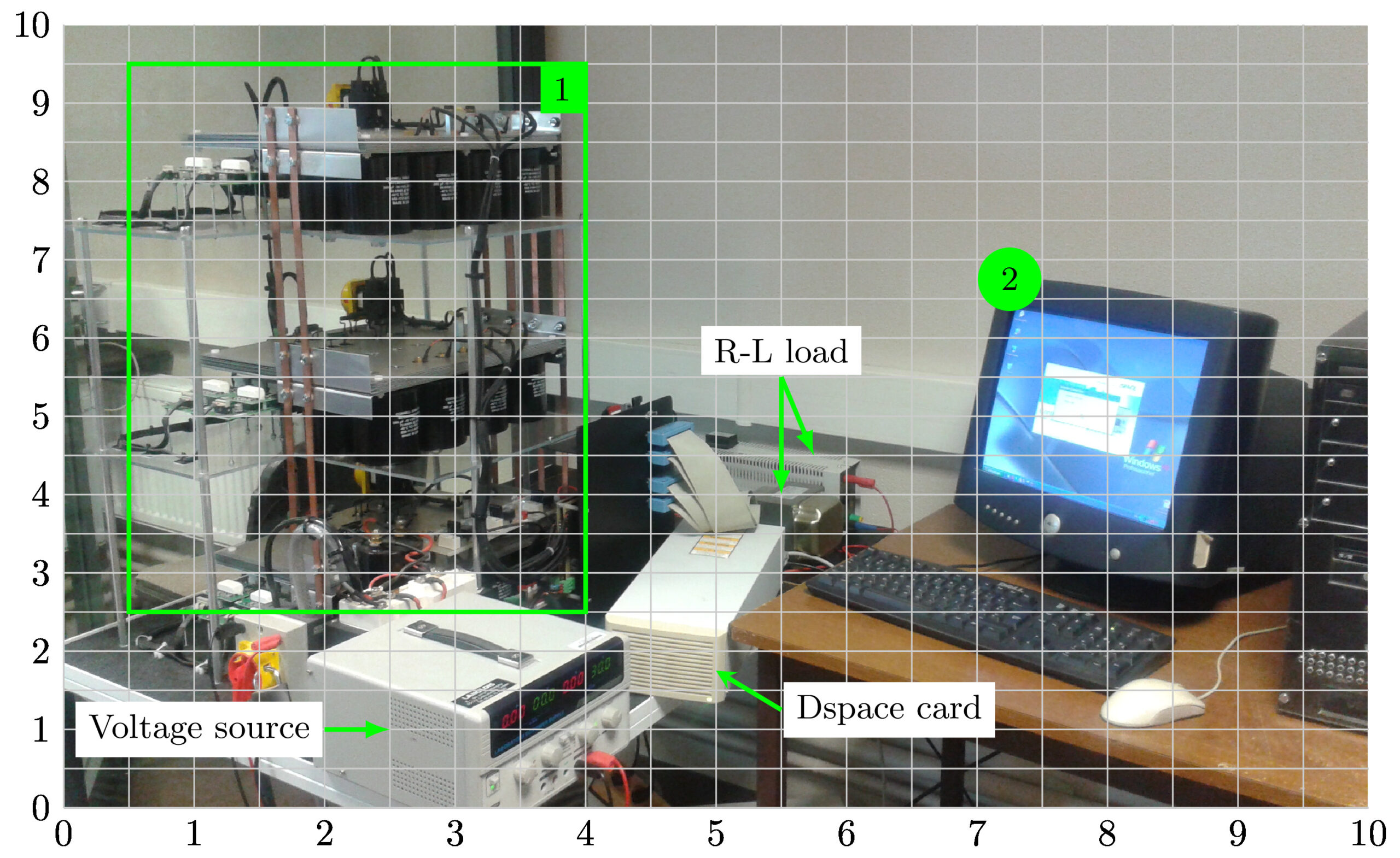
In this part, we will learn how to add different labels to annotate our illustration. Let's start by the first label "circled number".
The line code:
\node[circle,fill=green] at (7.25,6.75){\small 2};
adds a node at the point with coordinates (7.25,675). The node shape is a circle filled with a green color (check this post for predefined shapes and this post for predefined colors).
The line code:
\draw[stealth-, very thick,green] (5,1.75) -- ++(0.5,-0.5) node[right,black,fill=white]{\small Dspace card};
- draws a very thick arrow with a green color. The arrow tip style is specified by the option stealth-, we can use also latex-.
- stealth- means the arrow tip is on the starting point of the straight line, -stealth means that the arrow tip is on the end point and stealth-stealth means the straight line has arrow tips on both extremities.
- The arrow starts from the point with coordinates (5,1.75) and increased by 0.5 along the x-axis and decreased by 0.5 along the y-axis.
- We added a node on the right of the end point of the straight line (we used basic placement for that).
- The node contains a small text "Dspace card" which is written with black color.
By default, the node shape is a rectangle (we change it to a circle in the previous line code), we filled it with a white color using the option fill=white.
The line code:
\draw[latex-, very thick,green] (2.5,1) -- ++(-0.5,0) node[left,black,fill=white]{\small Voltage source};
adds the label "Voltage source" to the illustration. In this case, we used the arrow tip latex-.
The line code:
\draw[very thick,green] (0.5,2.5) rectangle (4,9.5) node[below left,black,fill=green]{\small 1};
- draws a rectangle from its two opposite corners ((0.5,2.5) and (4,9.5)).
- The rectangle is drawn with a green very thick line (check the next illustration about different options of line thickness).
- We added a node at the bottom left of the point (4,9.5). It is filled with green color and it has the rectangular shape (by default).
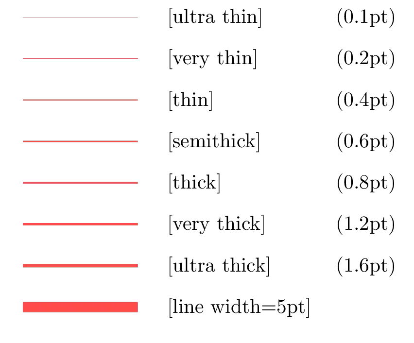
Line width options
Here is the code of the annotated image (you can comment the grid and axes' labels to get the final results). In the next section, we will highlight another method based on Pgfplots package.
Final code of step 3 (add labels, shapes and arrows):
 \documentclass{standalone}

\usepackage{tikz}
\usetikzlibrary{calc}

\begin{document}

\begin{tikzpicture}

% Include the image in a node
\node [
	above right,
	inner sep=0] (image) at (0,0) {\includegraphics[width=\textwidth]{example-image}};

% Create scope with normalized axes
\begin{scope}[
x={($0.1*(image.south east)$)},
y={($0.1*(image.north west)$)}]

% Grid
	\draw[lightgray,step=1] (image.south west) grid (image.north east);

% Axes' labels
	\foreach \x in {0,1,...,10} { \node [below] at (\x,0) {\x}; }
	\foreach \y in {0,1,...,10} { \node [left] at (0,\y) {\y};}

% Labels
	\node[circle,fill=green] at (7.25,6.75){\small 2};

	\draw[latex-, very thick,green] (2.5,1) -- ++(-0.5,0)
		node[left,black,fill=white]{\small Voltage source};

	\draw[stealth-, very thick,green] (5,1.75) -- ++(0.5,-0.5)
		node[right,black,fill=white]{\small Dspace card};

	\draw[very thick,green] (0.5,2.5) rectangle (4,9.5)
		node[below left,black,fill=green]{\small 1};

	\draw[latex-, very thick,green] (5.5,4) edge (5.5,5.5)
		(5.75,4.5) -- (5.5,5.5)
		node[above,black,fill=white]{\small R-L load};
\end{scope}

\end{tikzpicture}

\end{document}
Can we do the same using Pgfplots?
I published a post about plotting functions in LaTeX using Pgfplots, I deeply invite you to check it. Besides plotting functions and data, Pgfplots package has the feature to include external graphics. The above annotated image is recreated using Pgfplots package and here is the LaTeX code:
 \documentclass{standalone}

\usepackage{pgfplots}
\pgfplotsset{compat = newest}

\begin{document}

\begin{tikzpicture}

\begin{axis}
[
	xmin = 0, xmax = 10,
	ymin = 0, ymax = 10,
	width =\textwidth,
	height =0.6\textwidth,
	scale only axis,
	grid = both,
	axis on top,
	%hide axis
]

% Add the image
\addplot graphics[xmin=0,ymin=0,xmax=10,ymax=10] {ExpSetup};

% Labels
	\node[circle,fill=green] at (axis cs:7.25,6.75){\small 2};

	\draw[latex-, very thick,green] (axis cs:2.5,1) -- ++(-0.5,0)
		node[left,black,fill=white]{\small Voltage source};

	\draw[stealth-, very thick,green] (axis cs:5,1.75) -- ++(0.5,-0.5)
		node[right,black,fill=white]{\small Dspace card};

	\draw[very thick,green] (axis cs:0.5,2.5) rectangle (axis cs:4,9.5)
		node[below left,black,fill=green]{\small 1};

	\draw[latex-, very thick,green] (axis cs:5.5,4) edge (axis cs:5.5,5.5)
		(axis cs:5.75,4.5) -- (axis cs:5.5,5.5)
		node[above,black,fill=white]{\small R-L load};
\end{axis}

\end{tikzpicture}

\end{document}
Comments:
Inside the axis environment we created an axis with the options:
- xmin =0, xmax=10, ymin=0, ymax=10: to set axes min and max labels.
- width=\textwidth, height=0.6\textwidth: to fix the figure size
- scale only axis: to force the axis box to fills the above desired dimensions. Without this option, the figure size corresponds to the axis box, axes' ticks and x-y labels.
- grid=both: to add a grid to the axis box.
- axis on top: without this option the grid will be hidden by the image
- hide axis: this option should be commented to display the grid. once we annotate our illustration we will use this option to hide the axis box, ticks and the grid.
The image is added in Pgfplots using the line code:
\addplot graphics[xmin=0,ymin=0,xmax=10,ymax=10] {ExpSetup};
For now, we reached the end of this tutorial and I hope you learned something 
- How to superimpose data to a given graph provided in an image format.
- Useful packages for figures annotation in LaTeX such as tikz-imagelabels package and overpic package.
- Online LaTeX overlay generator.
If you have any remarks or suggestions, please feel free to use the comment section, I will be happy to hear from you!
Thanks and Stay safe!

There is a small mistake in the code: the two \foreach loops should be within scope environment.
You’re right, all labels and grid have to be inside the scope environment.
Thanks for your feedback, I really appreciate it 😊!
Thanks for the tutorials. These are the things to be really appreciated!
I am very grateful to your encouraging feedback!