Draw a Plane Intersecting a Cone in LaTeX

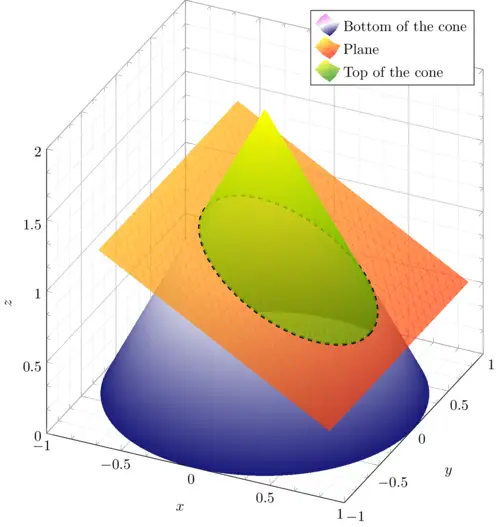
The illustration can be simplified to 5 pieces: 1) axes, 2) bottom part of the cone, 3) plane, 4) ellipse with dashed line style, 5) top part of the cone. These pieces have to be drawn in the correct order.

1. Set up the environment

First thing first, set up the environment according to the code below. Always remember to load the pgfplots package when it comes to plotting functions and data. Here we also use the colormaps library from the pgfplots package which allows us to change the gradient color of the surfaces.

The following code creates and customizes the plot (axes, labels, legend and plot size).  

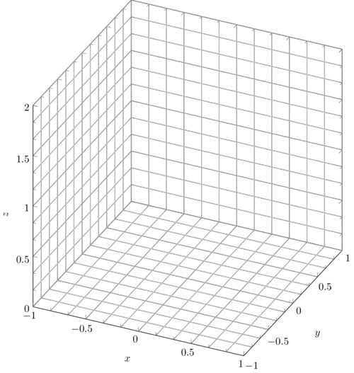
Compiling this code yields:

Comments:

In the options of the axis environment, we have added the following options:

- axis equal image: This options keeps an equal aspect ratio of the axis.

- grid = both: Plots the major and minor grid.

- grid style: Helps to change the default style of the grids like colours or stroke.

- label: Adds a name to the axis.

- legend cell align: Aligns the legend to the left, right or centre, we are going to see how it works at the end of the document.

- scale: Enlarges or stretches the graphics according with the parameter passed.

- z buffer = sort: Specify the way the pgfplots computes and orders the plots.

It is also important to set the limits of the graphic by the min and max commands, check this tutorial: How to plot a Function and Data in LaTeX.

Next step is to draw the bottom of the cone!

2. Draw the bottom of the cone

As we mentioned before, we are not going to explain or deduce where the parametric equation of the bottom of the cone comes from, instead we limit us to show what the equation is and show how to plot it.

The parametric equation of the bottom cone is given by :

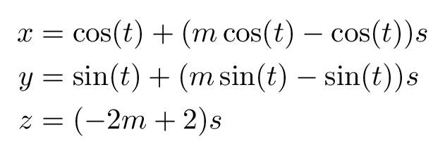
Where:

The parameter t takes values from [0, 2\pi] and the parameter s from [0, 1].

The above equation can be implemented as follows:

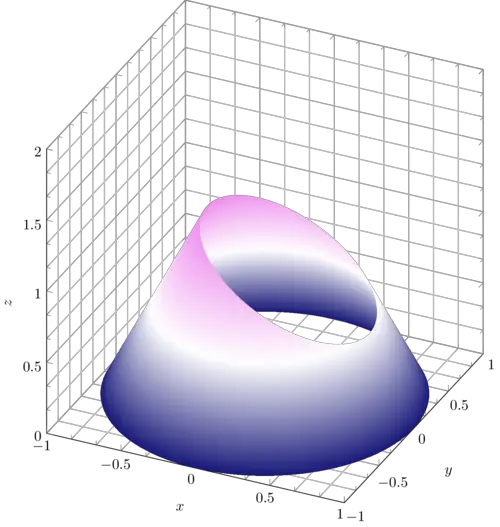
Adding this piece code to the above axis environment, we get the following result:

Comments: 

We have used the \addplot3 command to plot the parametric surface. Here are a description for the options used for this command:

- surf: Specifies that the plot is a surface.

- shader: It's the interpretation of the compiler, you can use inter for a smooth surface or flat for a rough one.

- samples: Defines the number of subdivisions for the surface.

- domain: Defines the domain of the parameter t and s, which are represented by x and y, respectively in the code above.

- colormap: Whit this command you can change the gradient color of the surfaces.

Once we have plotted the bottom of the cone, we can now plot the plane.

3. Draw the plane

In this part, we will do the same as the cone plot but with a different equation representing the plane.

 The equation of the plane is given by :

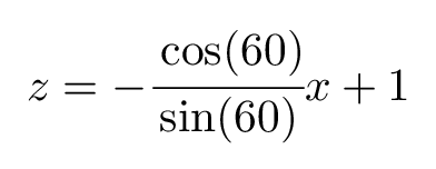
To plot the plane we can use again the \addplot3 command for the above equation:

Adding this piece of code under the previous \addplot3 of the cone's bottom part, we get the following illustration:

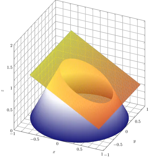
Again, it should be noted that the order is important. Otherwise, the plane will be drawn behind the cone. 

Let's move now to drawing the ellipse!

4. Draw an ellipse in 3D coordinates

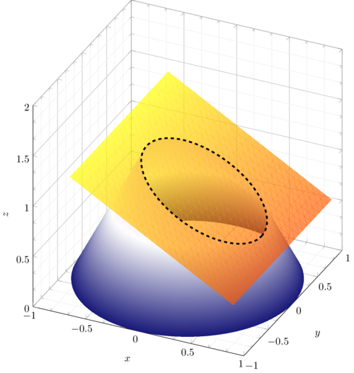
To highlight the intersection of the plane with the code, we need to draw an ellipse that can be described by a parametric curve. In this case, the parametric curve of the ellipse is given by:

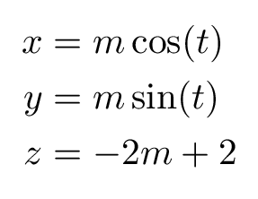
We can use the command \draw to plot a parametric equation. Check the code below:

5. Draw the top part of the cone

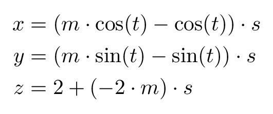
Finally, it remains to add the plot of the top of the cone. Once more time we need to add a 3D plot of a parametric surface described by the following equation:

Here is the final LaTeX code of a plane intersecting a cone:

Notice that we have added the line code:

 \legend{Bottom of the cone, Plane, Top of the cone}

which adds a box with the description of the surfaces at the top right of the graph. The legend text is aligned to the left by the option legend cell align={left} .