Plot Vector Field in LaTeX TikZ

A vector field is an assignment of a vector to each point in a subset of space with a given magnitude and direction. In this tutorial, we will learn how to draw vector field in 2-dimensional coordinates using TikZ and Pgfplots packages.

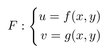
A vector field is a set of vectors in space, which every coordinate (x,y) has a vector of components [u,v]. The components of the vectors are functions of the coordinates, it means we can write the vector field as a mathematical expressions of the variables x and y:

TikZ provides the quiver option, which is a very useful way to plot vector fields. You may have heard about something similar if you are using Matlab. Let’s see how it is working in LaTeX !

1. Create tikzpicture environment

First you have to set up the LaTeX document where we need to load Pgfplots package. The latter loads automatically the TikZ package. Here is the corresponding LaTeX code:

\documentclass{standalone}

\usepackage{pgfplots}

\pgfplotsset{compat=newest}

\begin{document}

\begin{tikzpicture}[]
	% Here goes the code
\end{tikzpicture}

\end{document}

2. Plot vector field in LaTeX

Consider the following example:

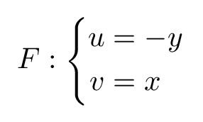
The following code shows how the option quiver is used to plot vector field of the above example:

\documentclass{standalone}

\usepackage{pgfplots}
\pgfplotsset{compat = newest}

\begin{document}

\begin{tikzpicture}
\begin{axis}[
	xmin = -4, xmax = 4,
	ymin = -4, ymax = 4,
	zmin = 0, zmax = 1,
	axis equal image,
	view = {0}{90},
]
	\addplot3[
		quiver = {
			u = {-y},
			v = {x},
		},
		-stealth,
		domain = -4:4,
		domain y = -4:4,
	] {0};
\end{axis}
\end{tikzpicture}

\end{document}

which yields the following illustration:

- In general the \addplot3 command is used to plot 3D surfaces, but we can modify it to get 2D representation of a vector field by writing down 0 at the end of the command. This means we are plotting the vector field in the xy plane.

- The -stealth option defines the type of arrow we want for the vectors, check this post for more options.

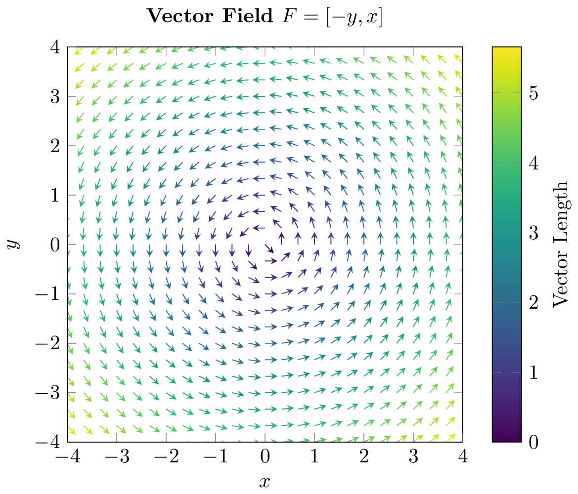
The obtained illustration after compiling this code is shown above. This vector field looks like a twister. Here we have settled a domain from -4 to 4. It’s important to set the visualization to view = {0}{90}, to get a projection on the xy plane.

Plotting a vector field is pretty easy! however, it requires little modification to get the desired results. The first issue is vectors are intersecting, and for better visualization we should normalize these vectors in order to avoid nasty intersections. And this the objective of the next section!

3. Normalize vectors

To normalize means to divide each vector by its modulus (the length of the vector). In this case the modulus of each vector is defined by:

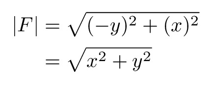
So if we divide each vector by its modulus, we will get a better representation of the vector field. Check the following code to get an idea about how we can do that in LaTeX:

\documentclass{standalone}

\usepackage{pgfplots}
\pgfplotsset{compat = newest}

\begin{document}

\begin{tikzpicture}
\begin{axis}[
	xmin = -4, xmax = 4,
	ymin = -4, ymax = 4,
	zmin = 0, zmax = 1,
	axis equal image,
	view = {0}{90},
]
	\addplot3[
		quiver = {
			u = {-y/sqrt(x^2+y^2)},
			v = {x/sqrt(x^2+y^2)},
			scale arrows = 0.25,
		},
		-stealth,
		domain = -4:4,
		domain y = -4:4,
	] {0};
\end{axis}
\end{tikzpicture}

\end{document}

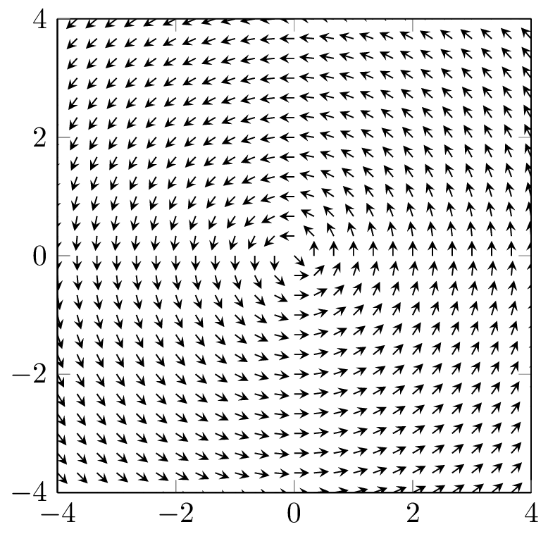
- Sometimes vectors are bigger than what we would like, for this reason it is recommended that we add a scaling factor to vectors by using the scale arrows =<value> command.

The obtained result is shown above. Now the vector field looks better, but we have lost some information about the real length of vectors. To solve this, we can use colormap to show the length of different vectors.

4. Add colormap to vector field

To use a colormap for the plot, we need to load the colormaps library in the preamble: \usepgfplotslibrary{colormaps}. This will load the default colormaps, so you can use them in your plots by writing colormap/color_map_name.

\documentclass{standalone}

\usepackage{pgfplots}
\pgfplotsset{compat = newest}
\usepgfplotslibrary{colormaps}

\begin{document}

\begin{tikzpicture}
\begin{axis}[
	xmin = -4, xmax = 4,
	ymin = -4, ymax = 4,
	zmin = 0, zmax = 1,
	axis equal image,
	xtick distance = 1,
	ytick distance = 1,
	view = {0}{90},
	scale = 1.25,
	title = {\bf Vector Field $F = [-y,x]$},
	height=7cm,
	xlabel = {$x$},
	ylabel = {$y$},
	colormap/viridis,
	colorbar,
	colorbar style = {
		ylabel = {Vector Length}
	}
]

\addplot3[
	point meta = {sqrt(x^2+y^2)},
	quiver = {
		u = {-y/sqrt(x^2+y^2)},
		v = {x/sqrt(x^2+y^2)},
		scale arrows = 0.25,
	},
	quiver/colored = {mapped color},
	-stealth,
	domain = -4:4,
	domain y = -4:4,
] {0};

\end{axis}

\end{tikzpicture}

\end{document}

The code shows how to implement the colormap and how to plot the colorbar by using these options in the \addplot3 command:

- point meta = \sqrt(x^2+y^2): This option sets the color of each vector in function of its length.
- quiver/colored: activates the colormap for the plot, if you don’t use this option you will generate a single color vector field.

And for the axis environment we use these options:

- colormap/viridis: here you can use any of the default colormaps provided by pgfplots like viridis, greenyellow, jet, hot and so on..
- colorbar: Shows a colorbar code at the right of the plot.

Also we have added labels for the axis and a title for the draw.

Using this example as a reference you can plot any vector field and use a colormap to make it look attractive without losing information of the length of each vector. That's all for today!

1. Create tikzpicture environment

2. Plot vector field in LaTeX

3. Normalize vectors

4. Add colormap to vector field

2 thoughts on “Plot Vector Field in LaTeX TikZ”