A phase portrait of a dynamical system is a geometric representation that depicts the system's trajectories in the phase plane. In this tutorial, we will learn how to draw the phase portrait of Van-Der-Pol oscillator in LaTeX using TikZ and Pgfplots.
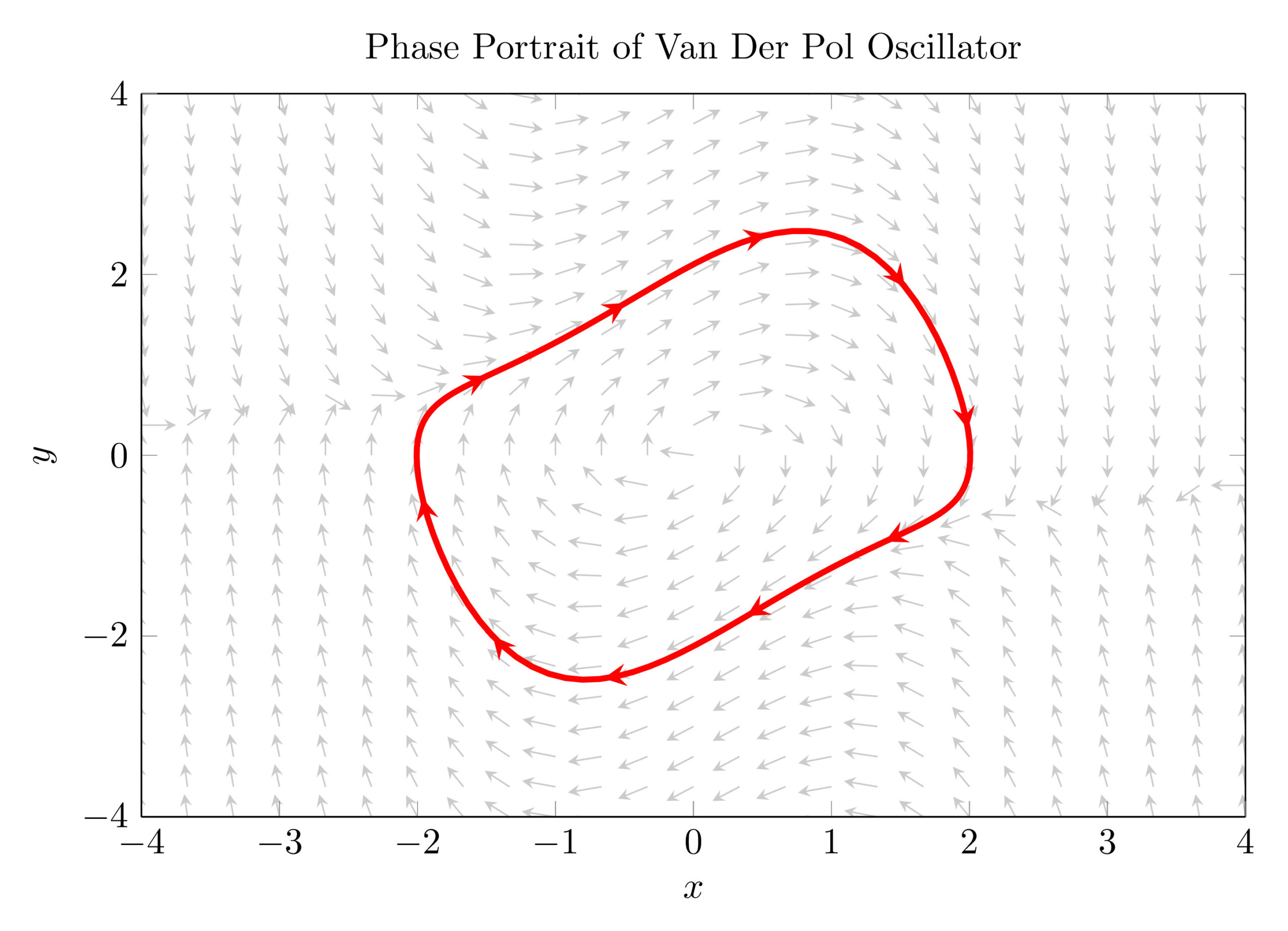
Let's start by the Limit Cycle
The Van der Pol oscillator can be represented by the following differential equations:
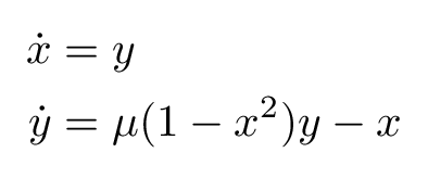
where μ is a scalar parameter indicating the damping strength. For μ, the nonlinear system has a stable limit cycle. However, it doesn't have an analytic solution that we can plot it directly in LaTeX using PGFplots package 

1. Solve the differential equations of the Van der Pol oscillator numerically (e.g. Matlab, python).
2. Export the solution as a table of x and y.
3. Plot it in LaTeX using PGFplots package .
1. Plot data using Pgfplots
In my case, I used Matlab/Simulink to simulate Van der Pol equations for μ=0.8. Then, I exported the solution (x and y) to the workspace of Matlab and extracted steady state data that corresponds to the limit cycle trajectory.
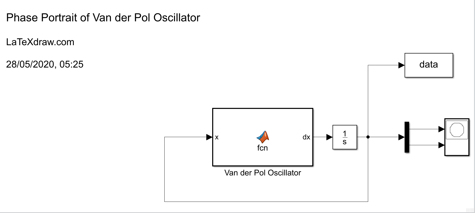
N.B. I used Matlab R2018a. Let me know if you need to export it to a previous version. Download Van der Pol Simulink file!
The next LaTeX code plots the limit cycle from an external file, named data.txt, using the \addplot command.
 \documentclass[border=0.2cm]{standalone}

\usepackage{pgfplots}
\pgfplotsset{compat = newest}

\begin{document}
\begin{tikzpicture}
\begin{axis}[
	grid=both,
	grid style={dashed,red!20},
	xmin = -4, xmax = 4,
	ymin = -4, ymax = 4,
	width = \textwidth,
	height = 0.7\textwidth,
	xlabel = {$x$},
	ylabel = {$y$},
	title={Phase Portrait of Van Der Pol Oscillator}
]

% Plot the Limit Cycle
\addplot[ultra thick, red] file {data.txt};

\end{axis}
\end{tikzpicture}

\end{document}
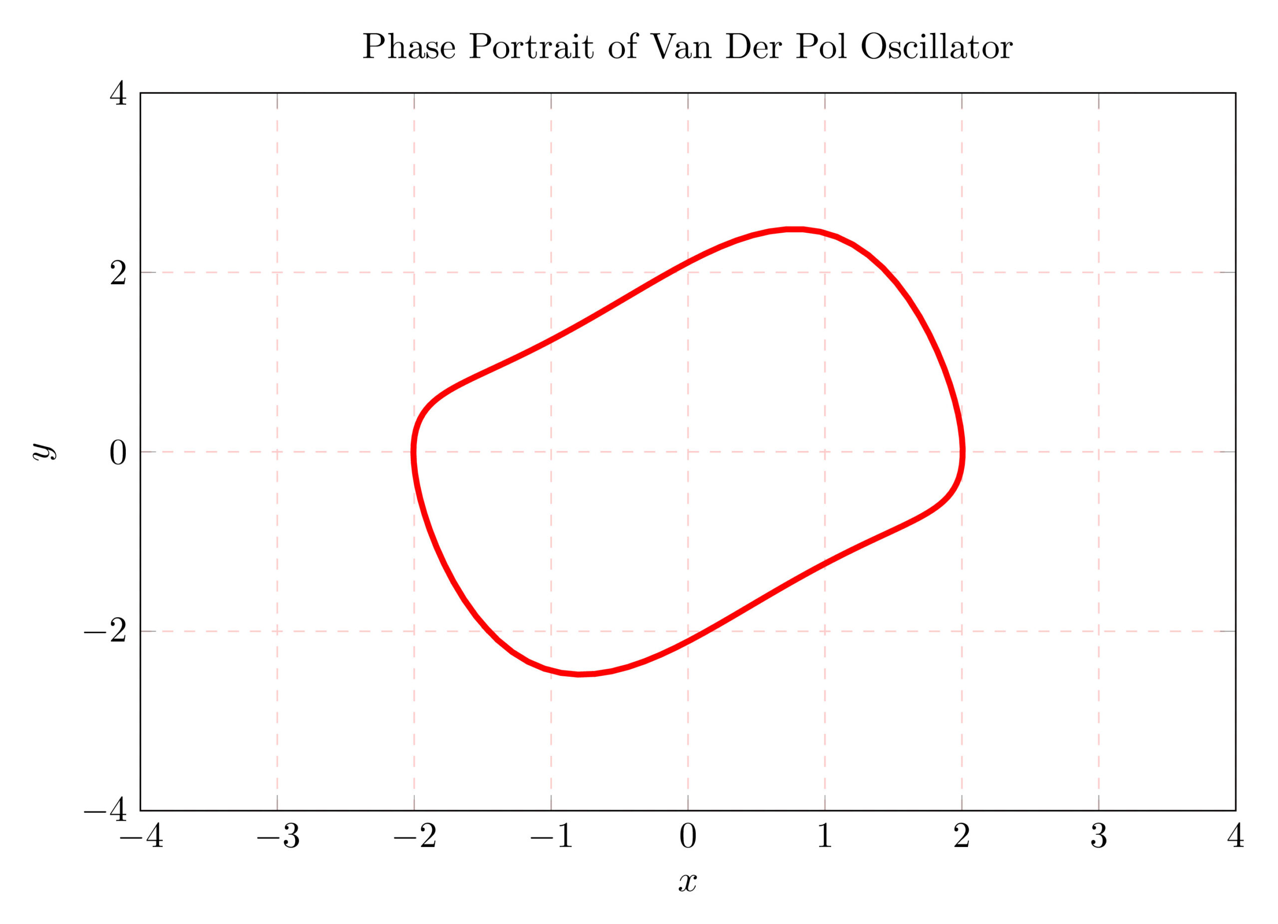
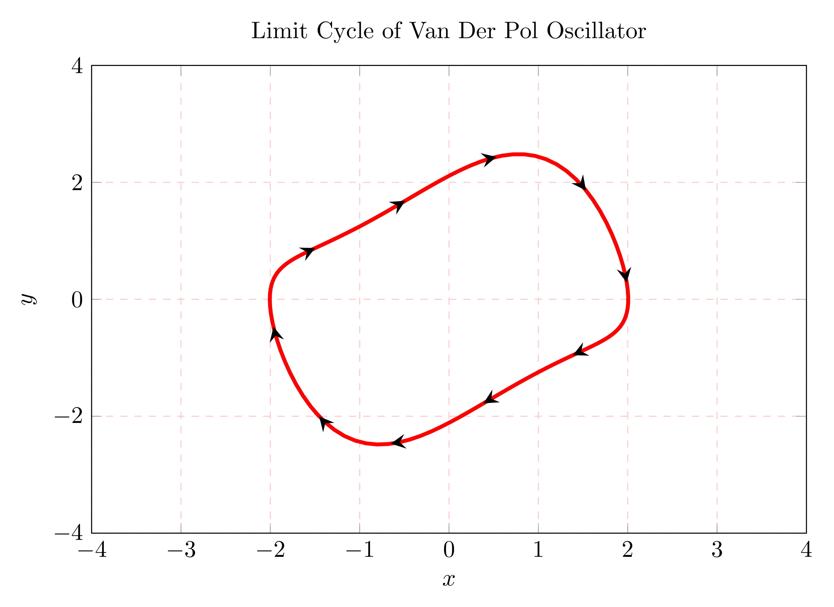
It should be noted that we plotted the state y in function of the state x but we need to highlight the evolution direction using small arrows.
2. Draw an arrow along a path
In the previous tutorial, "How to draw an arrow in the middle of a line in TikZ?", we have presented different methods that can be used in order to add an arrowhead along a path. We will use method 2 based on decorations.markings library (repeated arrows case). Inspired by this post, A slight modification is considered.
 \documentclass[border=0.2cm]{standalone}

\usepackage{pgfplots}
\pgfplotsset{compat = newest}

% Define arrow's style
\usetikzlibrary{decorations.markings}

\tikzset{decorated arrows/.style={
	postaction={
		decorate,
		decoration={
			markings,
			mark=between positions 0 and 1 step 15mm with {\arrow[black]{stealth};}
			}
		},
	}
}

\begin{document}
\begin{tikzpicture}

\begin{axis}[
	grid=both,
	grid style={dashed,red!20},
	xmin = -4, xmax = 4,
	ymin = -4, ymax = 4,
	width = \textwidth,
	height = 0.7\textwidth,
	xlabel = {$x$},
	ylabel = {$y$},
	title={Limit Cycle of Van Der Pol Oscillator}
]

% Plot the Limit Cycle
\addplot[ultra thick, red, decorated arrows] file {data.txt};

\end{axis}
\end{tikzpicture}

\end{document}
Comments:
- A TikZ style, named decorated arrows, is created using \tikzset command.
- It creates repetitive arrows between 0 (start of the path) and 1 (end of the path). A 15mm distance between successive arrows.
- Arrowhead style is chosen stealth with black color.
- The created style (decorated arrows) is add as an option to \addplot which draws the path in question.
3. Plot trajectories (transient and steady states)
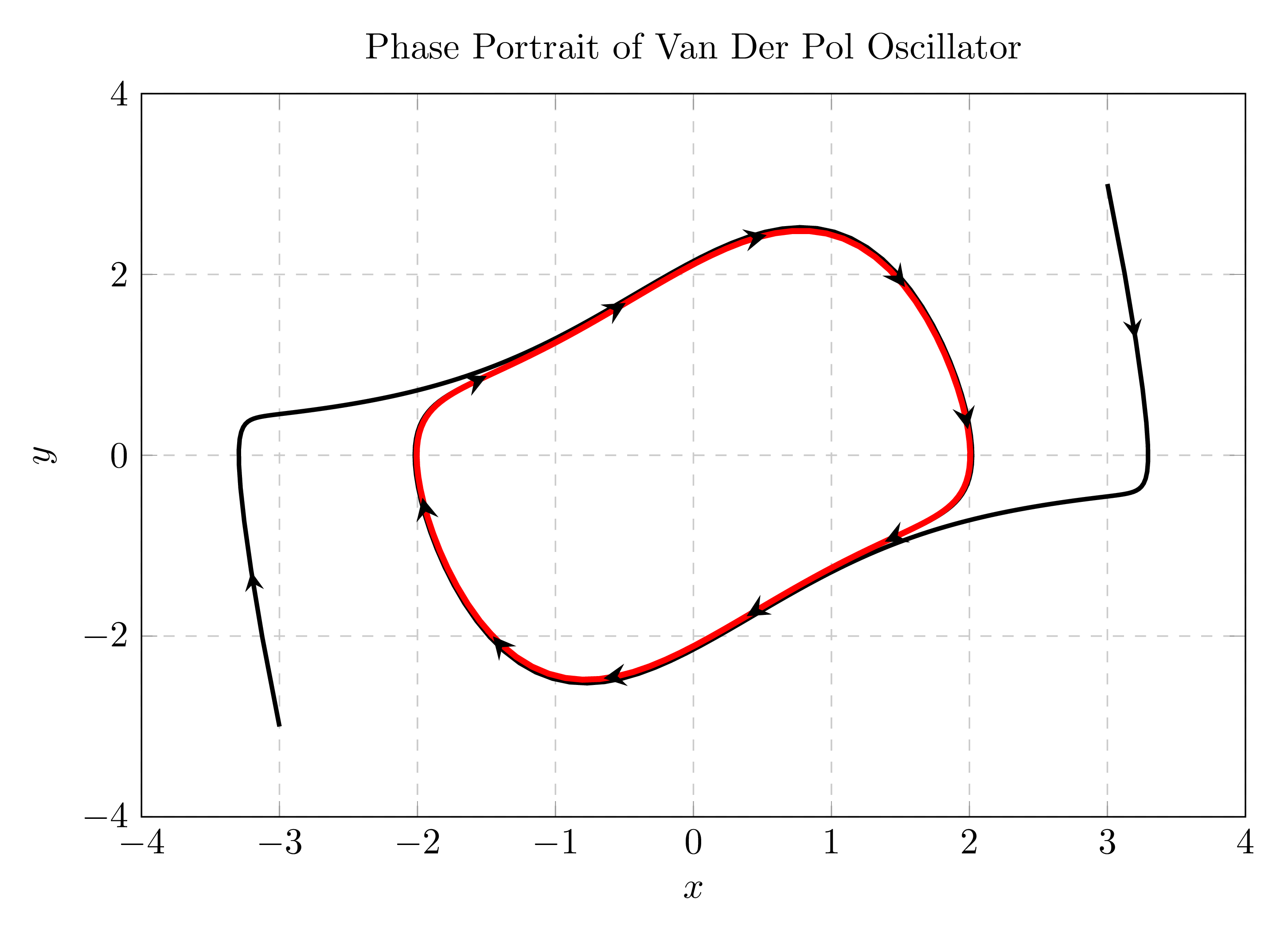
In the previous subsection, we plotted the limit cycle of Van der Pol oscillator, which is obtained by removing the transient part of the system's trajectory (this works as we are dealing with a stable limit cycle). To add trajectories starting from different initial conditions, we will follow the same steps as above. Here is an example of two trajectories starting from different initial conditions outside the limit cycle:
 \documentclass[border=0.2cm]{standalone}

\usepackage{pgfplots}
\pgfplotsset{compat = newest}

% Define arrow's style
\usetikzlibrary{decorations.markings}

% Arrow style 1
\tikzset{decorated arrows/.style={
	postaction={
		decorate,
		decoration={
			markings,
			mark=between positions 0 and 1 step 15mm with {\arrow[black]{stealth};}
			}
		},
	}
}

% Arrow style 2
\tikzset{decorated arrows2/.style={
	postaction={
		decorate,
		decoration={
			markings,
			mark=at position 15mm with {\arrow[black]{stealth};}
			}
		},
	}
}


\begin{document}
\begin{tikzpicture}

\begin{axis}[
	grid=both,
	grid style={dashed},
	xmin = -4, xmax = 4,
	ymin = -4, ymax = 4,
	width = \textwidth,
	height = 0.7\textwidth,
	xlabel = {$x$},
	ylabel = {$y$},
	title={Phase Portrait of Van Der Pol Oscillator}
]

% Trajectories
\addplot[very thick, decorated arrows2] file {data1.txt};
\addplot[very thick, decorated arrows2] file {data2.txt};


% Plot the Limit Cycle
\addplot[ultra thick, red, decorated arrows] file {data.txt};

\end{axis}
\end{tikzpicture}

\end{document}
Comments:
- As trajectories converge to the limit cycle and to avoid too much arrows on the limit cycle's path, we decorated trajectories with only one arrow head, positioned at 15mm from the starting the point.
4. Plot Vector Field
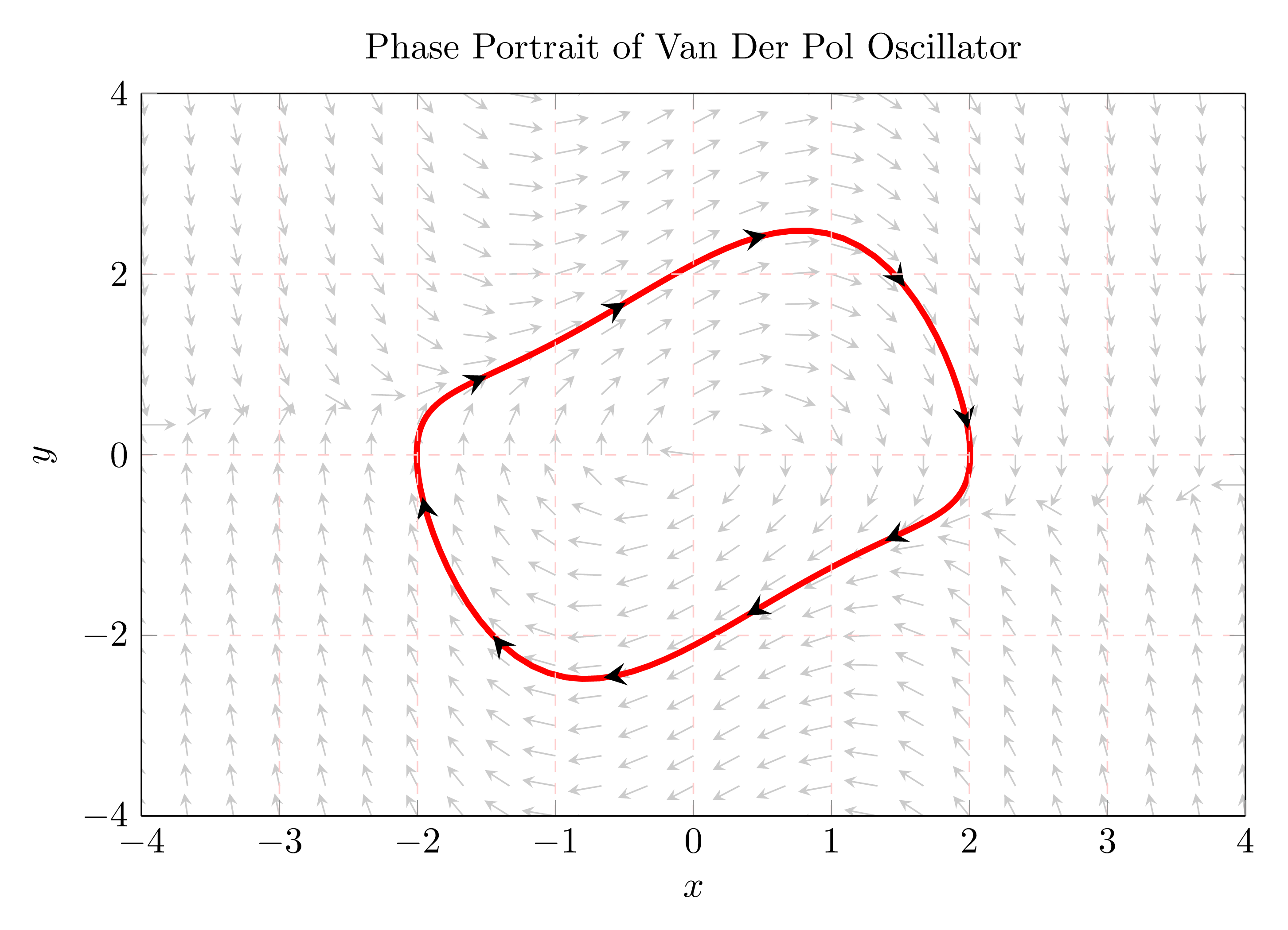
A vector field is an assignment of a small vector (with a given magnitude and direction) to each point in the phase plane. The direction and magnitude depends on the system dynamics.
A vector field can be drawn in LaTeX usign Pgfplots with quiver option. The first thing that we need is a set of points that fill the plane. Then we add small arrows, tangent to the system's trajectories, at each point.
You may wonder how one can create a set of points that fills the phase plane using Pgfplots? This can be achieved as follows:
1. Move to a 3D plot by using the command \addplot3;
2. Define x and y domains (-4 to 4 in this example)
3. Choose your function z=0, this will provides a set of points that fills the xy-plane with z=0
4. Change the view from 3D to a 2D version (xy plane)
Here is the corresponding code:
 \documentclass[border=0.2cm]{standalone}

\usepackage{pgfplots}
\pgfplotsset{compat = newest}

% Define arrow's style
\usetikzlibrary{decorations.markings}

% Arrow style
\tikzset{decorated arrows/.style={
	postaction={
		decorate,
		decoration={
			markings,
			mark=between positions 0 and 1 step 15mm with {\arrow[black]{stealth};}
			}
		},
	}
}


\begin{document}
\begin{tikzpicture}

\begin{axis}[
	grid=both,
	grid style={dashed,red!20},
	xmin = -4, xmax = 4,
	ymin = -4, ymax = 4,
	width = \textwidth,
	height = 0.7\textwidth,
	xlabel = {$x$},
	ylabel = {$y$},
	title={Phase Portrait of Van Der Pol Oscillator},
	view = {0}{90},
]

% Vector Field
\addplot3[
	quiver = {
		u = {y/sqrt(y^2+(0.8*(1-x^2)*y-x)^2)},
		v = {(0.8*(1-x^2)*y-x)/sqrt(y^2+(0.8*(1-x^2)*y-x)^2)},
		scale arrows = 0.25,
	},
	-stealth,
	domain = -4:4,
	domain y = -4:4,
	lightgray]
{0};

% Plot the Limit Cycle
\addplot[ultra thick, red, decorated arrows] file {data.txt};

\end{axis}
\end{tikzpicture}

\end{document}
Comments:
- The option view{0}{90} projects the plot into xy-plane.
- quiver is used as an option to \addplot3. We provide a normalized version of dx/dt and dy/dt to quiver.
- Normalized equations yields clean results with normalized vectors. Magnitude information is lost in this case but we can add a color mapping.
- Arrowhead style is chosen stealth .
We have reached the end of this tutorial, I hope you find it useful 
If you have any remarks or suggestions, do not hesitate to contact me, I will be happy to hear from you!
Thanks!
