Filling an Area Between Two Curves

In this tutorial, we will learn how to fill the area between two plot lines in LaTeX using PGFplots package and fillbetween library. We will draw the axis, place the function plots and fill the area between them.

Table of Contents

1. Required packages and libraries

2. Plot and save paths

3. Fill area between saved paths

4. Coordinates in axis environment

Filling the area between two plots can be achieved easily as follows:
1) draw the first plot and save its name by the option name path = <name>,
2) draw the second plot and save it with the same manner,
3) Use fill between operation (provided by fillbetween library).

Let's get into the detail!

1. Required packages and libraries

Plotting functions and data in LaTeX can be achieved by PGFplots package. Filling the area between two plots requires loading fillbetween library. The following code shows how one can load these element in LaTeX:

\documentclass[border=0.2cm]{standalone}

% Required Package and Librarie
\usepackage{pgfplots}
\pgfplotsset{compat=newest}
\usepgfplotslibrary{fillbetween}

\begin{document}

\begin{tikzpicture}
	% Illustration code
\end{tikzpicture}

\end{document}

2. Plot and save paths

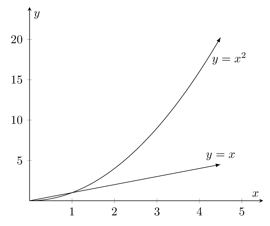
Let's consider the case of plotting the following functions:

The following code draws these functions in the domain [0,4.5]:

\documentclass[border=0.2cm]{standalone}

% Required Package and Librarie
\usepackage{pgfplots}
\pgfplotsset{compat=newest}
\usepgfplotslibrary{fillbetween}

\begin{document}

\begin{tikzpicture}
\begin{axis}[
	axis lines = middle,
	xlabel = {$x$},
	ylabel = {$y$},
	xmin=0, xmax=5.5,
	ymin=0, ymax=24]

% Plot 1
\addplot [name path = A,
	-latex,
	domain = 0:4.5,
	samples = 1000] {x^2} 
	node [very near end, right] {$y=x^2$};

% Plot 2
\addplot [name path = B,
	-latex,
	domain = 0:4.5] {x} 
	node [pos=1, above] {$y=x$};

\end{axis}
\end{tikzpicture}

\end{document}

which yields:

Comments:

- Functions are drawn using \addplot command.

- Each plot ends with an arrow Tip which is achieved by adding the option -latex to the \addplot command, Check TikZ arrows for more styles.

- Text labels are added to both plots using the \node command.

- The first plot is saved as A using the option name path=A with \addplot command. The second plot is saved as B using the option name path=B with \addplot command.

- For more details, I invite you to check this introduction to plotting functions and data in LaTeX.

3. Fill area between saved paths

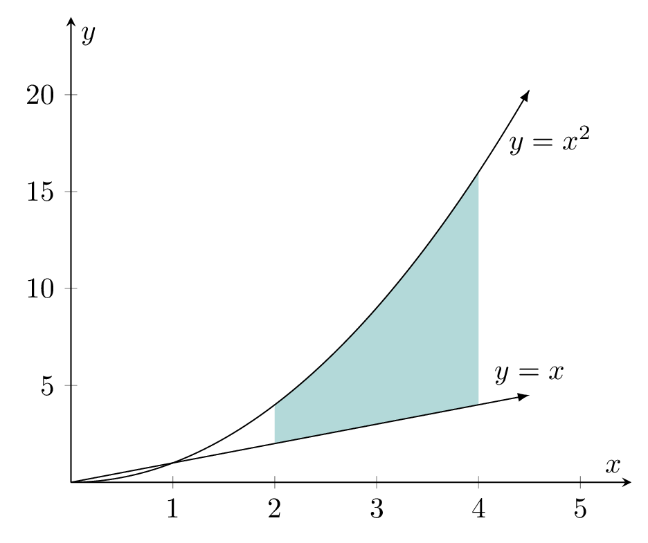
To fill the area between these curves, we can use fill between command with of = A and B option. We also place a soft clip here, since we want to only fill between 2 and 4. Here is the extended LaTeX code:

\documentclass[border=0.2cm]{standalone}

% Required Package and Librarie
\usepackage{pgfplots}
\pgfplotsset{compat=newest}
\usepgfplotslibrary{fillbetween}

\begin{document}

\begin{tikzpicture}
\begin{axis}[
	axis lines = middle,
	xlabel = {$x$},
	ylabel = {$y$},
	xmin=0, xmax=5.5,
	ymin=0, ymax=24]

% Plot 1
\addplot [name path = A,
	-latex,
	domain = 0:4.5,
	samples = 1000] {x^2} 
	node [very near end, right] {$y=x^2$};

% Plot 2
\addplot [name path = B,
	-latex,
	domain = 0:4.5] {x} 
	node [pos=1, above] {$y=x$};

% Fill area between paths
\addplot [teal!30] fill between [of = A and B, soft clip={domain=2:4}];

\end{axis}
\end{tikzpicture}

\end{document}

which yields the following result:

Filling an area between two plots TikZ Pgfplots

4. Coordinates in axis environment

You may wonder how to get axis environment coordinates in order to use them with TikZ commands. For example, I would like to add a text node at (1,20) with respect to axis environment, How to do it?

Answer: this can be achieved using the coordinate syntax: (axis cs:{1,20}).

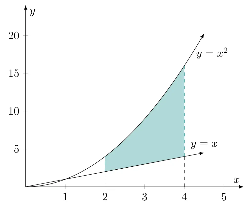
Final LaTeX code of filling area between the plot of the two functions:

\documentclass[border=0.2cm]{standalone}

% Required Package and Librarie
\usepackage{pgfplots}
\pgfplotsset{compat=newest}
\usepgfplotslibrary{fillbetween}

\begin{document}

\begin{tikzpicture}
\begin{axis}[
	axis lines = middle,
	xlabel = {$x$},
	ylabel = {$y$},
	xmin=0, xmax=5.5,
	ymin=0, ymax=24]

% Plot 1
\addplot [name path = A,
	-latex,
	domain = 0:4.5,
	samples = 1000] {x^2} 
	node [very near end, right] {$y=x^2$};

% Plot 2
\addplot [name path = B,
	-latex,
	domain = 0:4.5] {x} 
	node [pos=1, above] {$y=x$};

% Fill area between paths
\addplot [teal!30] fill between [of = A and B, soft clip={domain=2:4}];

% Dashed lines
\draw [dashed, teal] (axis cs:{2,2}) -- (axis cs:{2,4});
\draw [dashed, teal] (axis cs:{4,4}) -- (axis cs:{4,16});
\draw [dashed] (axis cs:{2,0}) -- (axis cs:{2,2});
\draw [dashed] (axis cs:{4,0}) -- (axis cs:{4,4});

\end{axis}
\end{tikzpicture}

\end{document}

Compiling this code yields to the following TikZ illustration:

Mainly, we have added dashed lines with different colors (teal and black). These lines are drawn the above coordinate syntax.

We've reached the end of this tutorial. If you have any questions or remarks, leave me a comment below or reach me via e-mail at admin@latexdraw.com, I will be happy to hear from you!