This tutorial is about drawing an electric field of an infinite line charge in LaTeX using TikZ package.
At the same time, we would like to show how to draw an arrow in the middle of a line or at any predefined position and use foreach loop for repeated shapes.
Updated post: we add a 3D version of the electric field using 3D coordinates in TikZ.

Step1: draw simple cylindrical shape in TikZ
The line charge is represented with a cylindrical shape which can be drawn by the mean of 2 straight lines, 2 arcs and and an ellipse as follows:

It should be noted that for geometry simplification, we draw the cylindrical shape (and different arrows) in an horizontal position then we will rotate it to get the final results.
Here is the corresponding LaTeX code of the cylindrical shape:
 \documentclass[border=0.2cm]{standalone}

\usepackae[dvipsnames]{xcolor}
\usepackage{tikz}

\begin{document}

\begin{tikzpicture}

% Cylindrical shape
\draw [top color=NavyBlue,
		bottom color=NavyBlue,
		middle color=Cyan] (0,-0.5) -- ++(12,0)
arc(-90:90:0.2 and 0.5) -- ++(-12,0)
arc(90:-90:0.2 and 0.5)--cycle;

\draw[fill=cyan!10] (0,0) ellipse(0.2 and 0.5);

\end{tikzpicture}

\end{document}
Comments:
- We start from the point with coordinates (0,-0.5) and we draw an horizontal straight line of 12cm length. Then, we add an arc that starts from -90 degrees and ends at 90 degrees with x-radius equals to 0.2cm and y-radius equals to 0.5cm. After that, we draw a straight line back (-12cm along the x-axis) using relative coordinates. Finally, we close the path by an arc that starts from 90 degrees and ends at -90 degrees.
- The previous shape is shaded by defining top, middle and bottom colors. It should be noted that we used predefined colors (dvipsnames).
- We added an ellipse filled with cyan!10 and has the same size as the drawn arcs (x-radius equals to 0.2cm and y-radius equals to 0.5cm).
Step 2: add electric charge
In this step, we would like to add plus sign to represent positive charges. This can be achieved using a node command and a foreach loop as follows:
 \foreach \j in {1,3.5,7,11}
{
	\node at (\j,0){$+$};
}

The loop variable, named [latex]\verb|\j|[/latex], takes values from the set [latex]\verb|{1,3.5,7,11}|[/latex] which are used to define the x-coordinate, along the x-axis, of each node. Each node draws a plus sign at the defined position.
Step 3: draw the electric field
The electric field is represented by a set of straight lines labelled with an arrowhead to specify its direction. In this example, we would like to draw a set of 18 arrows: 12 arrows behind the cylindrical shape (has to be drawn first) and 6 arrows above the cylindrical shape (has to be drawn last).

Each arrow is drawn by one line code and as we need to repeat this 18 times (different angles and different x coordinates) we will use a nested loop (a loop within a loop):
- one sets the x-coordinate value (1cm, 6cm and 11cm),
- the second sets the angle of the arrow.
Here is the corresponding code without rotation:
 \documentclass[border=0.2cm]{standalone}

\usepackage[dvipsnames]{xcolor}
\usepackage{tikz}
\usetikzlibrary{ decorations.markings}

\begin{document}

\begin{tikzpicture}
[decoration={markings,
		mark= at position 0.7 with {\arrow[line width=0.5mm]{latex}}}
]

% Electric Field (arrows of back layer)
\foreach \j in{1,6,11}
{
	\begin{scope}[xshift=\j cm]
		\foreach \angle in {90,150,210,270}
			{
				\draw[thick,postaction={decorate}] (\angle:0.4) -- (\angle:2.5);
			}
	\end{scope}
}

% Cylindrical shape
\draw [top color=NavyBlue,
			bottom color=NavyBlue,
			middle color=Cyan,
			opacity=0.92] (0,-0.5) -- ++(12,0)
	arc(-90:90:0.2 and 0.5) -- ++(-12,0)
	arc(90:-90:0.2 and 0.5)--cycle;

\draw[fill=cyan!10] (0,0) ellipse(0.2 and 0.5);

% Electric charge
\foreach \j in {1,3.5,7,11}
{
	\node at (\j,0){$+$};
}

% Electric Field (arrows of front layer)
\foreach \j in {0.75,5.75,10.75}
{
	\begin{scope}[xshift=\j cm]
		\foreach \angle in {-30,30}
			{
				\draw[thick,postaction={decorate}] (\angle:0.5) -- (\angle:2.5);
			}
	\end{scope}
}

\end{tikzpicture}

\end{document}
Comments:
- We used method 2 for drawing arrows in the middle of a line (check this post for more details).
- We used polar coordinates to draw different arrows, the angle is provided by a foreach loop variable.
- Arrowheads are positioned at 0.7 of the path length. For more shapes and style options, I deeply invite to read this post: Exploring TikZ arrows!
Step 4: geometric shape rotation in TikZ
Now, it remains to rotate the illustration by 10 degrees. This can be achieved by putting the illustration code inside a scope with the option transform canvas={rotate=10}.
 \documentclass[border=0.2cm]{standalone}

\usepackage[dvipsnames]{xcolor}
\usepackage{tikz}
\usetikzlibrary{ decorations.markings}

\begin{document}

\begin{tikzpicture}
[decoration={markings,
	mark= at position 0.7 with {\arrow[line width=0.5mm]{latex}}}
]

% Solve rotation issue
\draw[white] (-2,-3) rectangle (13.5,5.25);

% Rotate the illustration
\begin{scope}[transform canvas={rotate=10}]

% Electric Field (arrows of back layer)
\foreach \j in{1,6,11}
{
	\begin{scope}[xshift=\j cm]
		\foreach \angle in {90,150,210,270}
			{
				\draw[thick,postaction={decorate}] (\angle:0.4) -- (\angle:2.5);
			}
	\end{scope}
}

% Cylindrical shape
\draw [top color=NavyBlue,
				bottom color=NavyBlue,
				middle color=Cyan,
				opacity=0.92] (0,-0.5) -- ++(12,0)
	arc(-90:90:0.2 and 0.5) -- ++(-12,0)
	arc(90:-90:0.2 and 0.5)--cycle;

\draw[fill=cyan!10] (0,0) ellipse(0.2 and 0.5);

% Electric charge
\foreach \j in {1,3.5,7,11}
{
	\node at (\j,0){$+$};
}

% Electric Field (arrows of front layer)
\foreach \j in {0.75,5.75,10.75}
{
	\begin{scope}[xshift=\j cm]
		\foreach \angle in {-30,30}
			{
				\draw[thick,postaction={decorate}] (\angle:0.5) -- (\angle:2.5);
			}
	\end{scope}
}

\end{scope} % end scope of the illustration rotation
\end{tikzpicture}

\end{document}
Remark: To avoid facing issues when we use rotation or scaling with transform canvas, we can add a white rectangle around our illustration. Scaling can be achieved by adding the key scale=0.7 to the transform canvas: transform canvas={rotate=10,scale=0.7}.


Without scaling

With 0.7 scaling
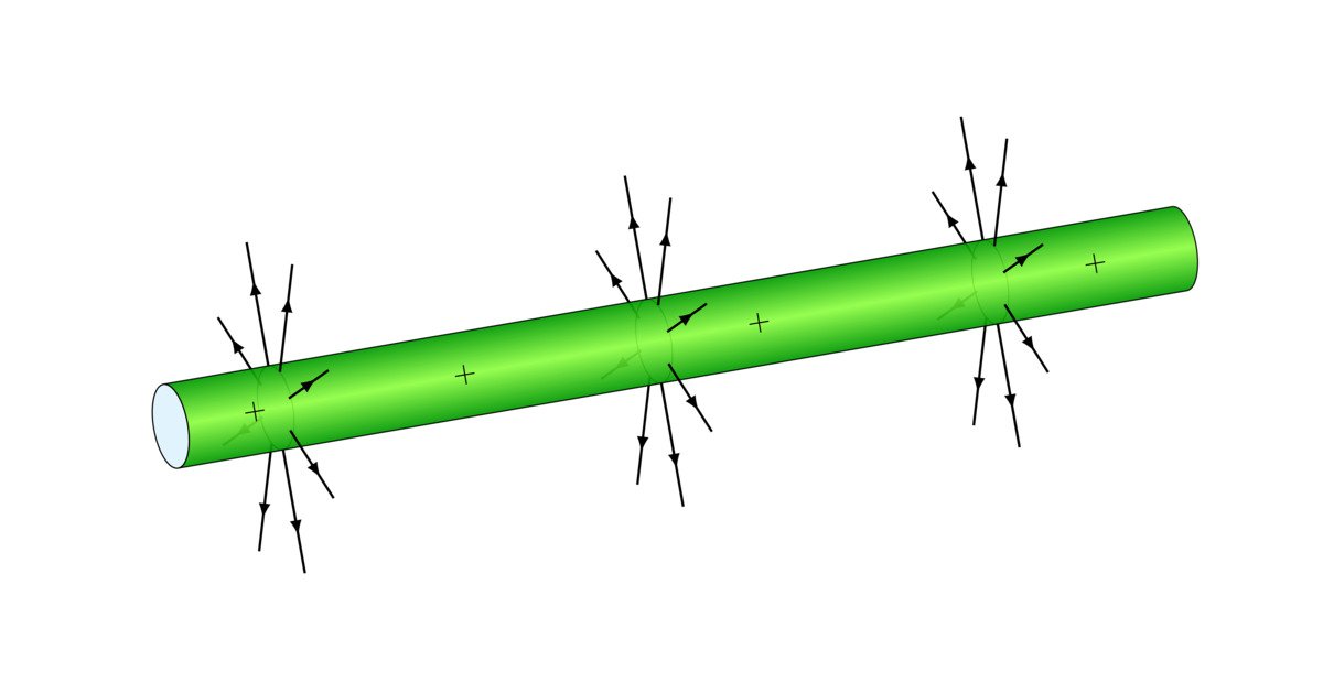
Update: Electric Field in 3D coordinates
You may remark that the current arrows do not seem to perfectly match the 3D orientation of the tube. To remedy this issue, we will use 3D coordinates for different arrows which start from an ellipse to create a 3D effect (check the images below). This is achieved using the package tikz-3dplot.


To draw these arrows, we use a nested loop:
- one sets the x-coordinate value (1.25cm, 5.75cm and 9.75cm), slightly modified compared to the previous values (1cm, 6cm and 11cm)
- the second sets the polar angle of the arrow in 3D coordinates.
The idea is to create two points (P1 and P2) with different radii: P1 on the surface of the tube with radius 0.5 cm, and P2 is set 2cm far from the center of the tube. This can be achieved in 3D coordinates using the command: \tdplotsetcoord{point}{r}{θ}{φ} where:
- point is the name of the coordinate (P1 or P2)
- r is the radius
- θ is the point polar angle
- φ is the point azimuthal angle
In our case, we will draw arrows with different polar angle. Here is the corresponding LaTeX code of the electric field of a line charge in 3D coordinates:
 \documentclass[]{standalone}

\usepackage[dvipsnames]{xcolor}
\usepackage{tikz}
\usepackage{tikz-3dplot}
\tdplotsetmaincoords{80}{70}

\usetikzlibrary{ decorations.markings}

\begin{document}

\begin{tikzpicture}
[decoration={markings,
	mark= at position 0.7 with {\arrow[]{latex}}}
]

% Solve rotation issue
\path[] (-2,-3) rectangle (13.5,5);

% Rotate the illustration
\begin{scope}[transform canvas={rotate=10}]

% Electric Field (arrows of back layer)
% 3D version

\foreach \j in {1.25,5.75,9.75}
{
\draw[xshift=\j cm] (0,0) ellipse(0.2 and 0.5);

\begin{scope}[xshift=\j cm,tdplot_main_coords]
	\foreach \angle in {0,45,...,180}
		{
			\tdplotsetcoord{P2}{2}{\angle}{-40}
			\tdplotsetcoord{P1}{0.5}{\angle}{-40}
			\draw[thick,postaction={decorate}] (P1) -- (P2);
}
\end{scope}
}

% Cylindrical shape
\draw [top color=NavyBlue,
			bottom color=NavyBlue,
			middle color=Cyan,
			opacity=0.92] (0,-0.5) -- ++(12,0)
	arc(-90:90:0.2 and 0.5) -- ++(-12,0)
	arc(90:-90:0.2 and 0.5)--cycle;

\draw[fill=cyan!10] (0,0) ellipse(0.2 and 0.5);


% Electric charge
\foreach \j in {1,3.5,7,11}
{
	\node at (\j,0){$+$};
}

% Electric Field (arrows of front layer)
% 3D version

\foreach \j in {1.25,5.75,9.75}
{
	\begin{scope}[xshift=\j cm,tdplot_main_coords]
		\foreach \angle in {180,225,...,360}
			{
				\tdplotsetcoord{P2}{2}{\angle}{-40}
				\tdplotsetcoord{P1}{0.5}{\angle}{-40}
				\draw[thick,postaction={decorate}] (P1) -- (P2);
			}
	\end{scope}
}

\end{scope} % end scope of the illustration rotation

\end{tikzpicture}

\end{document}
Special thanks!
Thank you guys for your encouraging feedback, your suggestions and comments on each published post. I have received a request from Sebastian to write a tutorial about drawing standard electromagnetic situations and this post is part of it.
Feel free to contact me, I will be happy to hear from you  !
!