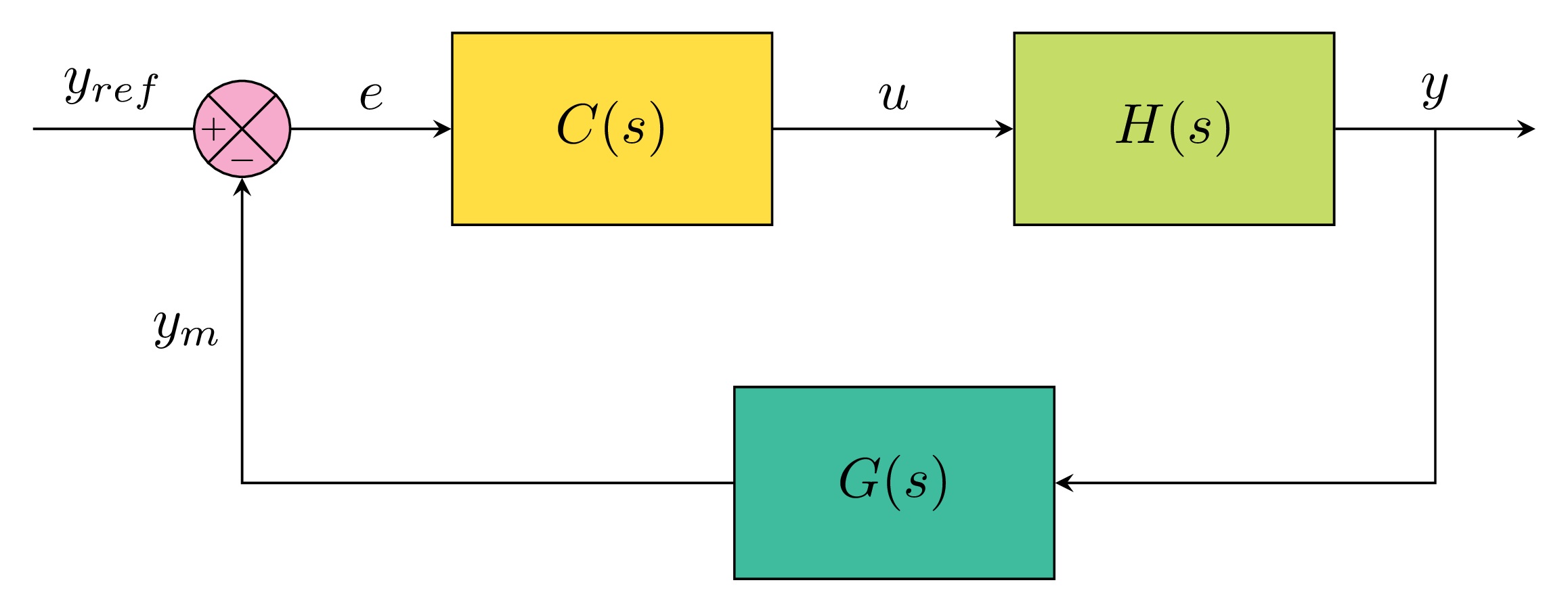

Block diagram drawn in LaTeX using TikZ package
Create nodes in TikZ
In our example, we distinguish two types of shapes: a circle and 3 rectangles. These shapes can be created using \node command. Here is an example:
\documentclass[border=0.2cm]{standalone}

% More defined colors
\usepackage[dvipsnames]{xcolor}

% Required package
\usepackage{tikz}
\usetikzlibrary{positioning}


\begin{document}

\begin{tikzpicture}

\node[draw,
	circle,
	minimum size=0.6cm,
	fill=Rhodamine!50
] (sum) at (0,0){};

\end{tikzpicture}

\end{document}
The above code creates a node with name (sum) at the point with coordinates (0,0). To draw the node, we have to add the option draw to it and with circle option, we get a circle shape. By default, a node corresponds to a rectangle.
We provided also the minimum size of the node which is equal to 0.6cm. It should be noted that adding details to a node (text, image or even a tikz code) increases its size.
The node is filled with the color Rhodamine!50 which is one of the dvipsnames provided by xcolor package. For a full list, check the post: Predefined LaTeX colors: dvipsnames.
Anchors of a node in TikZ
Each node has anchors which corresponds to points coordinates of the node border. A feature that is not provided by draw command with circle shape. Different anchors are shown in the next illustration where we use the name of the node and an angle or we use predefined anchors such as (north, south, east, west, etc)

Now, we can draw easily the sum shape of the block diagram by connecting the point (sum.north east) with the point (sum.south west) through a straight line using draw command. The same for the points with coordinates (sum.south east) and (sum.north west). Here is the code:
\documentclass[border=0.2cm]{standalone}

% More defined colors
\usepackage[dvipsnames]{xcolor}

% Required package
\usepackage{tikz}
\usetikzlibrary{positioning}


\begin{document}

\begin{tikzpicture}

% Sum shape
\node[draw,
	circle,
	minimum size=0.6cm,
	fill=Rhodamine!50
] (sum) at (0,0){};

\draw (sum.north east) -- (sum.south west)
	(sum.north west) -- (sum.south east);

\end{tikzpicture}

\end{document}
which yields the following illustration:

Now, it remains to add the positive and negative signs. We can place them as nodes relative to the center of the sum node. Here is the corresponding piece of code:
\node[left=-1pt] at (sum.center){\tiny $+$};
\node[below] at (sum.center){\tiny $-$};
Adding these two lines to the previous code, we get the following result:

We added the option left=<value> to put the node at the left of the provided coordinates (sum.center) with an offset equals to the provided value. The same for the negative sign which is located below the center of the sum node.
Relative positioning in TikZ
Now, we would like to create the controller block which corresponds to a rectangle filled with a golden color and has the label C(s). This can be achieved following the same steps as above where we will create a node with draw option and specify its size. To avoid positioning the at specific coordinates (x,y), we will use relative positioning with respect to the sum node. Check the following code:
\documentclass[border=0.2cm]{standalone}

% More defined colors
\usepackage[dvipsnames]{xcolor}

% Required package
\usepackage{tikz}
\usetikzlibrary{positioning}


\begin{document}

\begin{tikzpicture}

% Sum shape
\node[draw,
	circle,
	minimum size=0.6cm,
	fill=Rhodamine!50
] (sum) at (0,0){};

\draw (sum.north east) -- (sum.south west)
	(sum.north west) -- (sum.south east);

\draw (sum.north east) -- (sum.south west)
(sum.north west) -- (sum.south east);

\node[left=-1pt] at (sum.center){\tiny $+$};
\node[below] at (sum.center){\tiny $-$};

% Controller
\node [draw,
	fill=Goldenrod,
	minimum width=2cm,
	minimum height=1.2cm,
	right=1cm of sum
]  (controller) {$C(s)$};

\end{tikzpicture}

\end{document}
The above code creates a node with rectangular shape (default shape no need to specify it) which has a minimum width =2cm and minimum height=2cm. The node is located at the right of the sum node with 1cm distance. This is achieved using the option right=1cm of sum. We saved the rectangle node with the name (controller) which will be used for relative positioning of the system block H(s). Here is the obtained illustration:

Following the same steps as above, we can create the system and the sensor blocks. Here is the corresponding code:
\documentclass[border=0.2cm]{standalone}

% More defined colors
\usepackage[dvipsnames]{xcolor}

% Required package
\usepackage{tikz}
\usetikzlibrary{positioning}


\begin{document}

\begin{tikzpicture}

% Sum shape
\node[draw,
	circle,
	minimum size=0.6cm,
	fill=Rhodamine!50
] (sum) at (0,0){};

\draw (sum.north east) -- (sum.south west)
	(sum.north west) -- (sum.south east);

\draw (sum.north east) -- (sum.south west)
(sum.north west) -- (sum.south east);

\node[left=-1pt] at (sum.center){\tiny $+$};
\node[below] at (sum.center){\tiny $-$};

% Controller
\node [draw,
	fill=Goldenrod,
	minimum width=2cm,
	minimum height=1.2cm,
	right=1cm of sum
]  (controller) {$C(s)$};

% System H(s)
\node [draw,
	fill=SpringGreen,
	minimum width=2cm,
	minimum height=1.2cm,
	right=1.5cm of controller
] (system) {$H(s)$};

% Sensor block
\node [draw,
	fill=SeaGreen,
	minimum width=2cm,
	minimum height=1.2cm,
	below right= 1cm and -0.25cm of controller
]  (sensor) {$G(s)$};

\end{tikzpicture}

\end{document}
Compiling this code yields:

The sensor is positioned at the right and below of the controller node using the option: below right= 1cm and -0.25cm of controller. It remains to connect these blocks with arrows.
Draw an arrow with text label
This is the easiest part in drawing a block diagram in LaTeX. We need to connect anchors of different nodes. Let's start by drawing an arrow between the sum and the controller blocks:
\draw[-stealth] (sum.east) -- (controller.west)
	node[midway,above]{$e$};
This line of code draws a line from (sum.east) to (controller.west). The line ends with an arrowhead of stealth type (For more arrow tips, check the post Exploring TikZ Arrows) . We added a label to the arrow using a node command, the label is positioned at the above the middle of the distance between two blocks. This has been achieved using midway option. The next table provides more details about positioning along a path:

We can do the same between the controller block and the system block:
\draw[-stealth] (controller.east) -- (system.west)
	node[midway,above]{$u$};
For the output of the system, we will draw an arrow with 1.25cm length and we save the node at the middle of the arrow to use it for connecting the output with sensor block. Here is the corresponding code:
\draw[-stealth] (system.east) -- ++ (1.25,0)
	node[midway](output){}
	node[midway,above]{$y$};
The node is named (output) and we will draw a line from its center (output.center) to the (sensor.east) with a perpendicular lines. To achieve the later, we use |- (vertical then straight line) instead of --.
\draw[-stealth] (output.center) |- (sensor.east);
\draw[-stealth] (sensor.west) -| (sum.south)
	node[near end,left]{$y_m$};
The west anchor of the sensor is connected with the south of the sum node using the path operation -| (straight then vertical line).
The input reference corresponds to a labeled arrow which can be drawn with the same manner as the output arrow.
Here is the Final code of the latex block diagram:
\documentclass[border=0.2cm]{standalone}

% More defined colors
\usepackage[dvipsnames]{xcolor}

% Required package
\usepackage{tikz}
\usetikzlibrary{positioning}


\begin{document}

\begin{tikzpicture}

% Sum shape
\node[draw,
	circle,
	minimum size=0.6cm,
	fill=Rhodamine!50
] (sum) at (0,0){};

\draw (sum.north east) -- (sum.south west)
	(sum.north west) -- (sum.south east);

\draw (sum.north east) -- (sum.south west)
(sum.north west) -- (sum.south east);

\node[left=-1pt] at (sum.center){\tiny $+$};
\node[below] at (sum.center){\tiny $-$};

% Controller
\node [draw,
	fill=Goldenrod,
	minimum width=2cm,
	minimum height=1.2cm,
	right=1cm of sum
]  (controller) {$C(s)$};

% System H(s)
\node [draw,
	fill=SpringGreen,
	minimum width=2cm,
	minimum height=1.2cm,
	right=1.5cm of controller
] (system) {$H(s)$};

% Sensor block
\node [draw,
	fill=SeaGreen,
	minimum width=2cm,
	minimum height=1.2cm,
	below right= 1cm and -0.25cm of controller
]  (sensor) {$G(s)$};

% Arrows with text label
\draw[-stealth] (sum.east) -- (controller.west)
	node[midway,above]{$e$};

\draw[-stealth] (controller.east) -- (system.west)
	node[midway,above]{$u$};

\draw[-stealth] (system.east) -- ++ (1.25,0)
	node[midway](output){}node[midway,above]{$y$};

\draw[-stealth] (output.center) |- (sensor.east);

\draw[-stealth] (sensor.west) -| (sum.south)
	node[near end,left]{$y_m$};

\draw (sum.west) -- ++(-1,0)
	node[midway,above]{$y_{ref}$};


\end{tikzpicture}

\end{document}Optimize the code with tikzstyle command
You may remarked that all rectangular blocks have the same dimension characteristics and to avoid repeating these options: draw, minimum width=2cm, minimum height=1.2cm, we can create a style with these options using the \tikzstyle command as follows:
\tikzstyle{block} = [
	draw,
	minimum width=2cm,
	minimum height=1.2cm
]
We named the style as block and we can use it as an option in all different node commands corresponding to the controller, system and sensor blocks.