Plot Step Response in TikZ: A Beginners’ Guide

What is a step response? 

In control theory, a step response is the time evolution of the system output when the input corresponds to a step.

Today's example is a first order system described by the following block diagram:

For a unit step and zero initial condition, the output of the system is given by the following equation:

In the sequel, we'll consider the case of K=7 and 𝜏=1.

Main elements of the plot

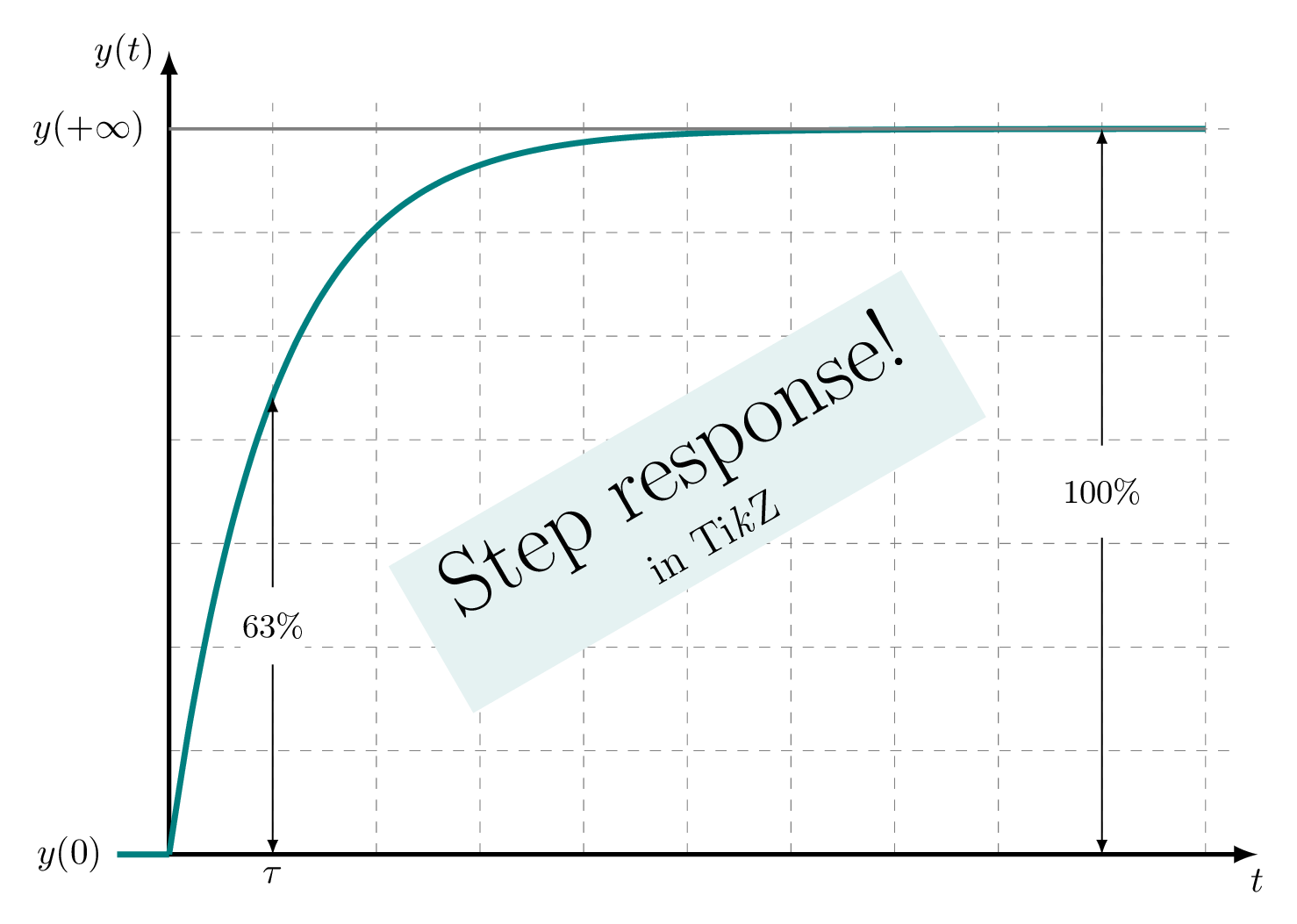
Here is the final result that we would like to get in LaTeX:

It can be simplified to small drawing tasks: 

1) The grid which has a dashed line style and light gray color. 

2) Axes which corresponds to a straight line ending with an arrowhead. Labels are added at the end points

3) Plot of a function with teal color and very thick line to distinguish it from the other parts.

4) Lines with arrowheads and a text label (63% & 100%) 

Let's see how this can be achieved using TikZ commands!

1. Create a grid in TikZ

Creating a grid in TikZ can be achieved with the same manner as drawing a rectangle where we need the coordinates of two opposite corners. Check the following code: 

Compiling this code yields:

Comments:

- Using the operation grid between the points (0,0) and (10.25,7.25), we have a created a grid with 10.25cm width and 7.25cm height.

- The option help lines yields thin and light gray style of the grid lines. 

- We have added dashed to get a dashed line style. 

- By default, the step between lines is 1cm and can be modified by these options: step=<value>, xstep=<value>, ystep=<value>. The first one sets the same step for vertical and horizontal lines. xstep (ystep) option sets the spacing between vertical (horizontal) lines, respectively. 

2. Add axes to the grid

Axes correspond to two perpendicular lines:

- The horizontal one representing x-axis starts from the point with coordinates (0,0) and ends at the point (10.5,0).

- The vertical line represents the y-axis and it starts from (0,0) and ends at the point (0,7.5). 

Check the following code:

And the corresponding illustration:

Comments:

- We used very thick option to change the line thickness

- The option -latex adds an arrowhead at the end of the line. latex- will add an arrowhead at the beginning of the line. You can guess what latex-latex will do! 

- More arrowhead styles and customization can be found in this post: TikZ arrows

- The node command will add the text between braces at the end point of the line. We added below and left options to position labels with respect to the end point. 

The two lines code of the axes can be minimized to only one line code using the operation |- (goes vertical than horizontal) instead of -- as follows:

Text nodes are added at the corresponding coordinates. Let's move to plotting our function!

3. Plot function in TikZ

Our function is equal to zero for t<0 and equal to the above equation for t>0. We will plot this function in the domain [-0.5, 10] and here is the corresponding the code: 

Compiling this code yields:

Comments:

- We added a text node, y(0), at the left of the starting point (-0.5,0)

- The code draws a straight line between the points (-0.5,0) and (0,0) using the operation --

- We used plot command to draw our function, described by the above equation, in the domain [0, 10]. This is achieved by the option domain=0:10

- samples =50 and smooth options yields to a smooth plot with 50 samples. 

4. Add arrows with midway labels

This can be done with the same manner as drawing the axes and we will add a node at the middle of the line with a white background. Here is how we can do it:

Compiling this code yields: