In this TikZ tutorial, we will learn how to plot a torus using its mathematical equations. To achieve this we will use Pgfplots, a pretty powerful package based on TikZ/PGF.
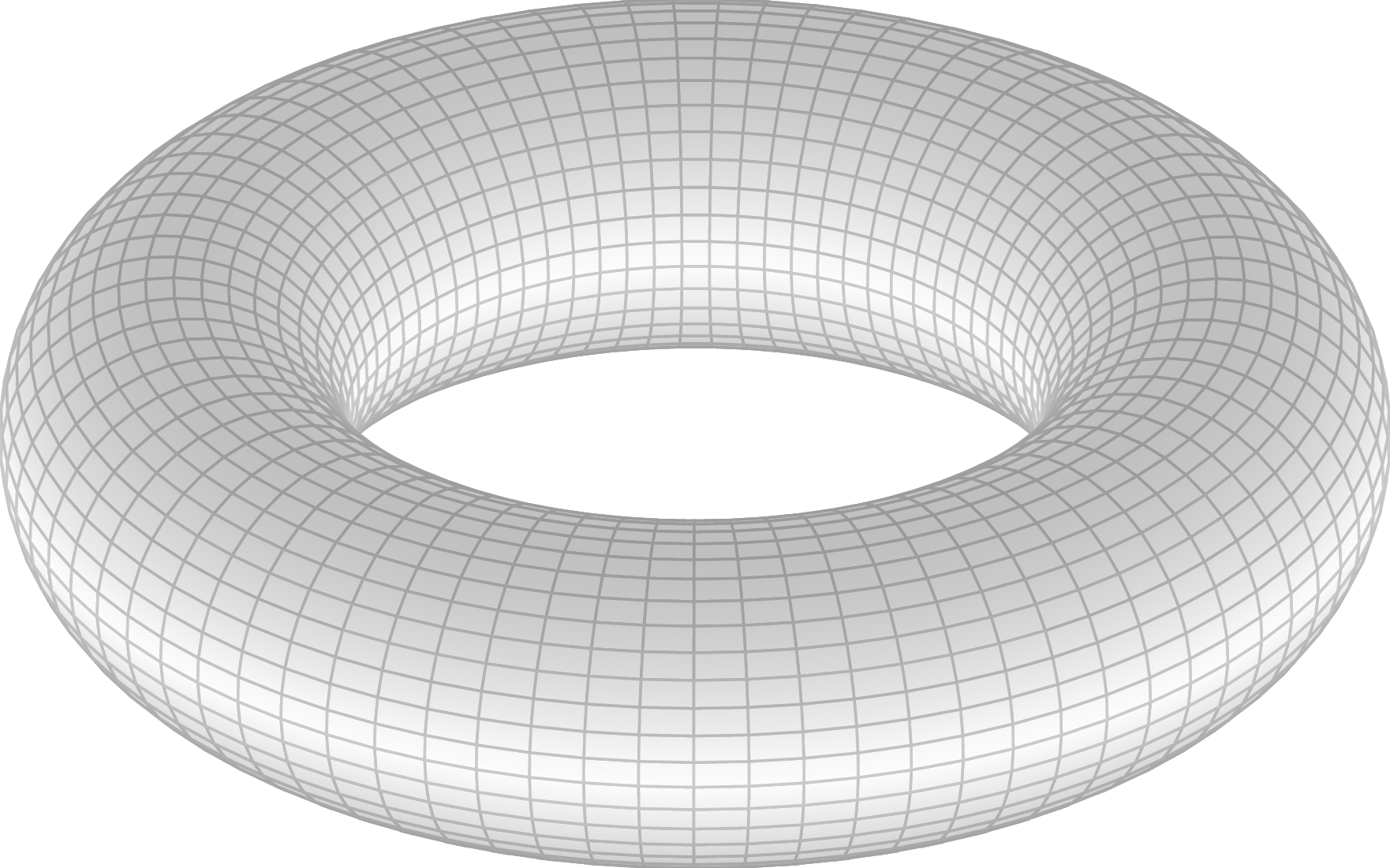
Parametric equation of a torus
A torus, pretty similar to a donut, can be plotted mathematically using the following parametric equation:
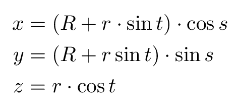
Where R is the external radius and r is the inner radius. The equation has the parameters t and s, which take values from 0 to 2π in order to plot the torus.
Required packages
Using TikZ we can plot any parametric equation. First we just need to set up the preamble in our LaTeX file as follows:
\documentclass{standalone}

\usepackage{tikz}
\usepackage{pgfplots}

\pgfplotsset{
	compat=newest
}

\begin{document}

\begin{tikzpicture}
	\begin{axis}[]
		% here comes all the code for drawing
	\end{axis}
\end{tikzpicture}

\end{document}
From the above code, we used the package TikZ and the package Pgfplots. The first one allows LaTeX to include vectorial illustrations in the document, and the second one is used to plot 2D curves or 3D surfaces. We mentioned above that Pgfplots is based on TikZ which means that loading Pgfplots is sufficient.
The command \pgfplotsset{compat=newest} sets the compatibility between packages to the last version developed.
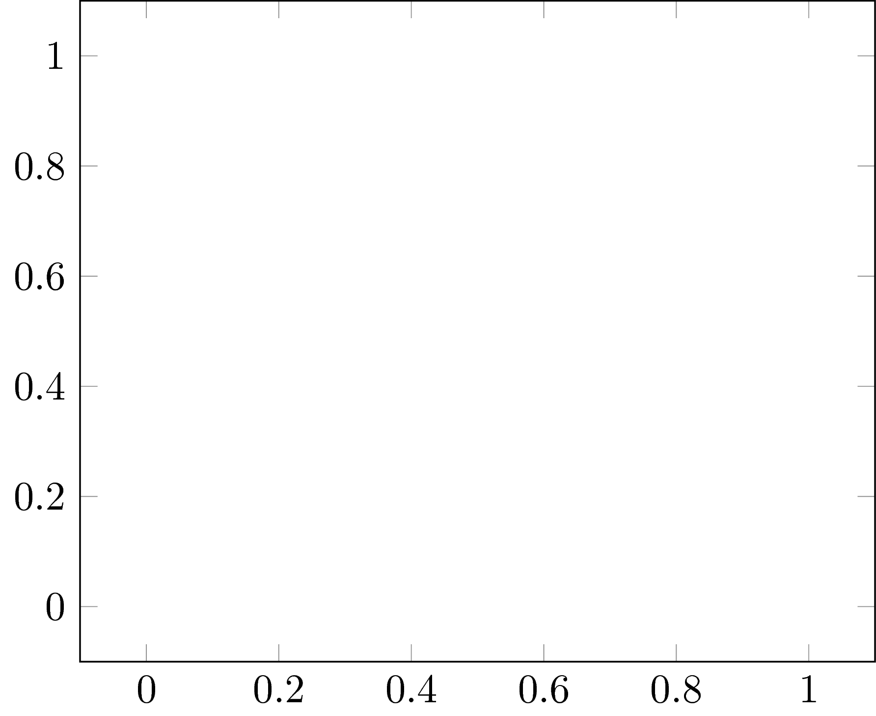
Inside the document environment, we distinguish two environments: tikzpicture and axis. All the code we are going to develop is going to be inside the axis environment. If you compile the code above you will get an empty coordinate system (see the next illustration).
Plot 3D functions in TikZ
In this part, we will use the command \addplot3[options](function) in order to get the plot of the parametric equation of the torus. If we set $R=1$ and $r=1$, we can plot the donut. Check the next code to figure out how the parametric equations should be typed.
\documentclass{standalone}

\usepackage{pgfplots}

\pgfplotsset{
	compat=newest
}

\begin{document}

\begin{tikzpicture}
	\begin{axis}[]
		\addplot3[](
			{(3+sin(deg(\x)))*cos(deg(\y))},
			{(3+sin(deg(\x)))*sin(deg(\y))},
			{cos(deg(\x))}
		);
	\end{axis}
\end{tikzpicture}

\end{document}
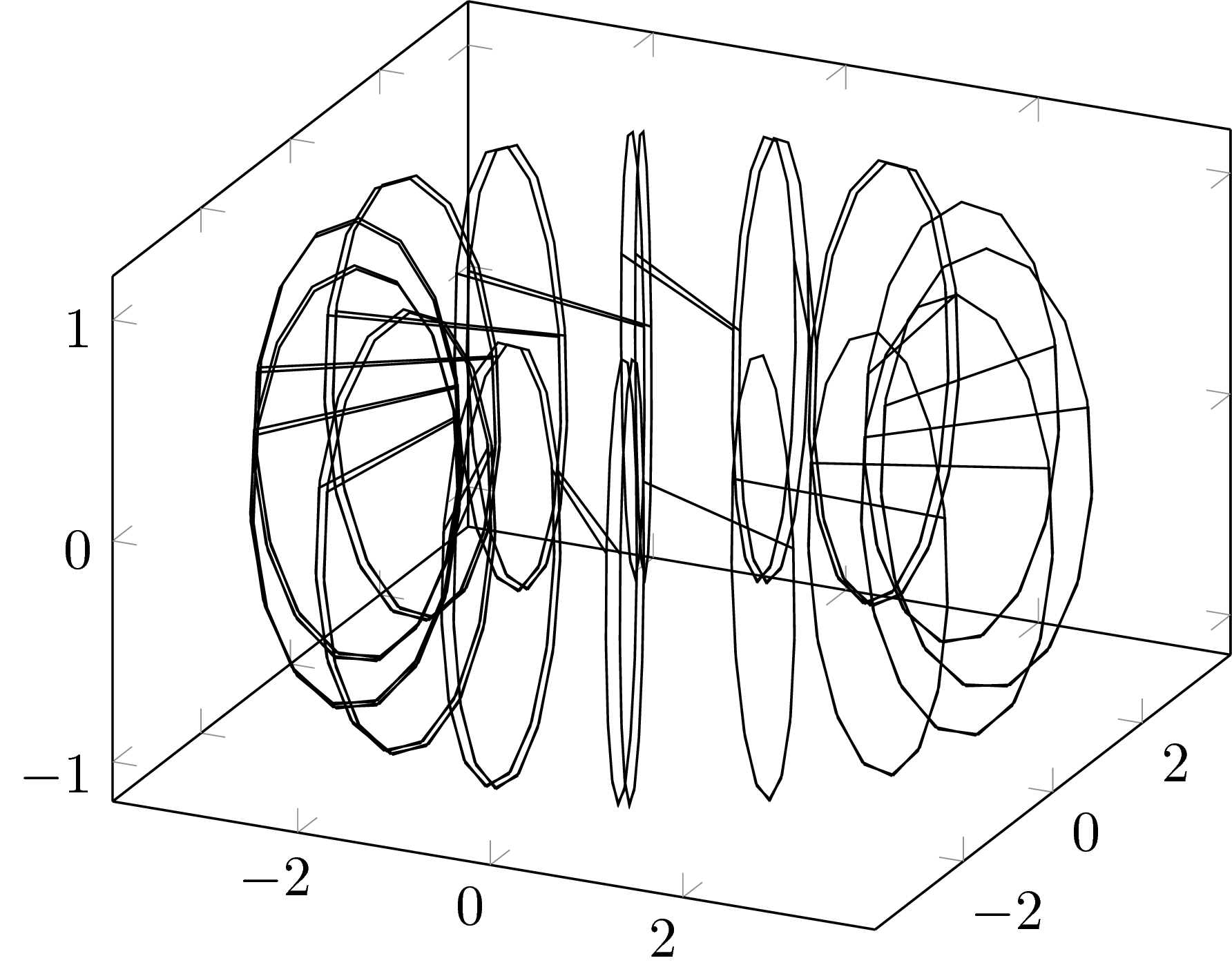
As you may figure out, the parameter t corresponds to x in the TikZ code, and s corresponds to y.
Now we see a 3D graphic, but it's far away from what we want. Note that the functions sin and cos requires angles in degrees, that's why we have to use the command deg(\x). Also notice that the options of the axis and the tikzpicture are empty. If we put the correct options we will get the desired shape. Let's add some options to the \addplot3 command.
\documentclass{standalone}

\usepackage{pgfplots}

\pgfplotsset{
	compat=newest
}

\begin{document}

\begin{tikzpicture}
	\begin{axis}[]
		\addplot3[
			surf,
			shader = faceted interp,
			samples = 40,
			samples y = 80,
			domain = 0:2*pi,
			domain y = 0:2*pi,
			thin,
		](
			{(3+sin(deg(\x)))*cos(deg(\y))},
			{(3+sin(deg(\x)))*sin(deg(\y))},
			{cos(deg(\x))}
		);
	\end{axis}
\end{tikzpicture}

\end{document}
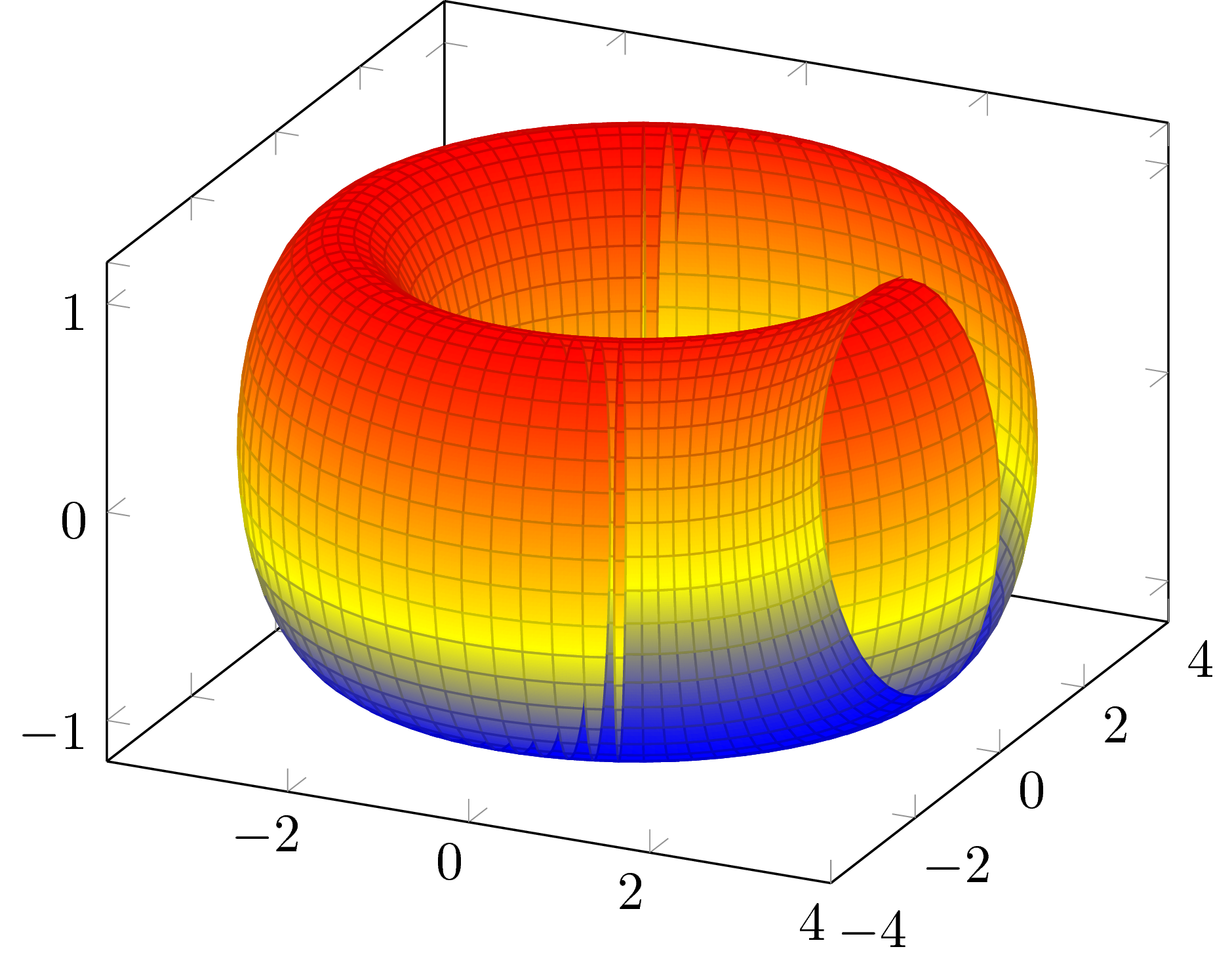
Comments:
- surf: defines the object as a surface.
- shader: determines the way the package computes the subdivision of the surface.
- samples: it's the number of subdivisions in the x and y direction.
- domain: represents the domain of the parameters s and t.
- thin: represents the stroke of the mesh over the surface.
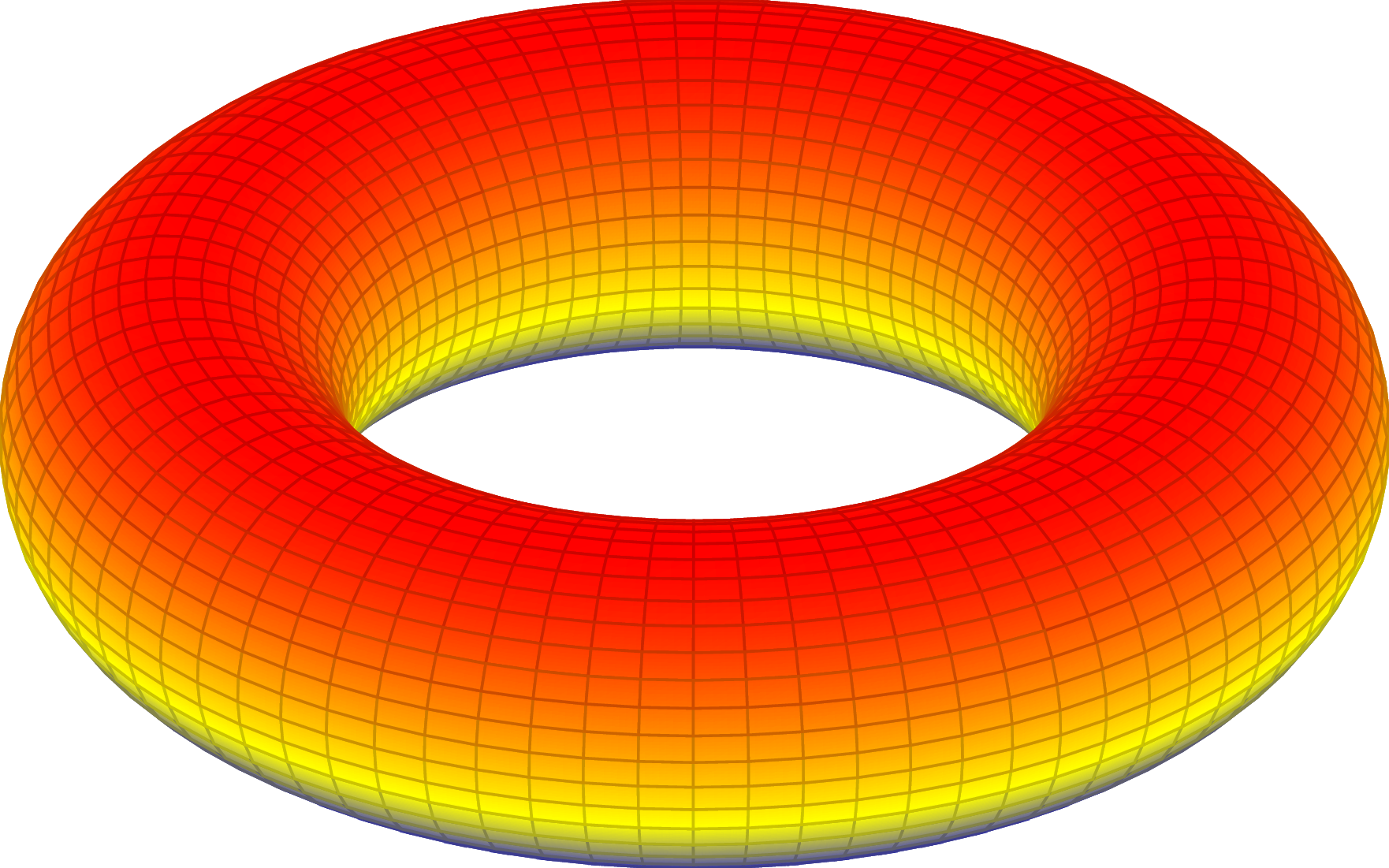
Now our torus looks better, but it's not enough. We can hide the axis, change the aspect ratio and make it look nicer in general. To achieve this, we have to set up some extra options in the axis environment, as follows:
\documentclass{standalone}

\usepackage{pgfplots}

\pgfplotsset{
	compat=newest
}

\begin{document}

\begin{tikzpicture}
	\begin{axis}[
		axis equal image,
		hide axis,
		z buffer = sort,
		view = {122}{30},
		scale = 1.5
	]
		\addplot3[
			surf,
			shader = faceted interp,
			samples = 40,
			samples y = 80,
			domain = 0:2*pi,
			domain y = 0:2*pi,
			thin,
		](
			{(3+sin(deg(\x)))*cos(deg(\y))},
			{(3+sin(deg(\x)))*sin(deg(\y))},
			{cos(deg(\x))}
		);
	\end{axis}
\end{tikzpicture}

\end{document}
Comments:
- axis equal image: sets the aspect ratio of the x, y and z as 1:1:1.
- hide axis: hides the referential coordinate system.
- z buffer: This command is very important when plotting 3D plots, it makes possible to render the surface with an accurate interpretation of the distribution of the mesh in space.
- view: sets the angle and orientation of the view.
- scale: scales the original size of the plot.
Customize the colormap
To put the final touch, let's give the torus some personality by changing the colour.
\documentclass{standalone}

\usepackage{pgfplots}
\usepgfplotslibrary{colormaps}

\pgfplotsset{
	compat=newest
	colormap={mycolormap}{color=(lightgray) color=(white) color=(lightgray)}
}

\begin{document}

\begin{tikzpicture}
	\begin{axis}[
		axis equal image,
		hide axis,
		z buffer = sort,
		view = {122}{30},
		scale = 1.5
	]
		\addplot3[
			surf,
			shader = faceted interp,
			samples = 40,
			samples y = 80,
			domain = 0:2*pi,
			domain y = 0:2*pi,
			colormap name = mycolormap,
			thin,
		](
			{(3+sin(deg(\x)))*cos(deg(\y))},
			{(3+sin(deg(\x)))*sin(deg(\y))},
			{cos(deg(\x))}
		);
	\end{axis}
\end{tikzpicture}

\end{document}

Just add the command colormap in the \pgfplotsset and choose the colour you want. Here we have a gray scheme, where the chosen colours are lightgray and white. Of course you can use the colours that you like. And we're done with our torus!
