Automata Diagrams in LaTeX

What is automata?

Automata is the plural form of automaton, which means self-making in Greek. They are used to define abstract computing devices, or machines, in a theoretical platform. Probably you only heard of them if you are studying automata theory, or have a theory of computation course in your curriculum. They are represented with state diagrams.

An automaton contains states and transitions. These states are usually drawn as a circle surrounding the state information. There are two special states:

- Initial state: is represented with an arrow that is pointing to the initial state

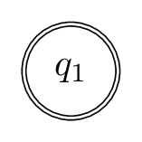
- Accepting states: are drawn with double lines

The initial state can also be an accepting state. All these states are connected with transitions, or arrows that shows how the input is carried around the automaton.

What we need to draw automata in LaTeX?

To get started, we need the following packages and libraries: 

 1. load TikZ package, the drawing package

 2. load automata library for drawing shapes easily, 

 3. arrows library to connect our states with special arrows, 

 4. positioning library to help position our states and transitions. 

We will declare them and then create a tikzpicture environment as follows:

Drawing an Automaton Diagram in TikZ

1. Create a state

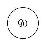
We can start drawing an automaton by creating our first state. In TikZ, we can use \node command to start drawing any shape. If we use it with state styling option that comes with the automata library, we will have our first state. Usually, states are named as q_0, q_1, etc. Let's draw our first state and name it q_0.

2. Absolute vs Relative positioning of a state

a. Absolute positioning of a state

We will go over absolute positions first. Our environment has a coordinate system, and the center point of the first node we draw is placed at point (0,0), by default.

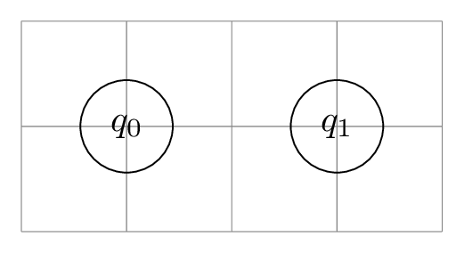
We can place a node to, let's say 2 cm right, by using at (2,0) command in our node definition. In the following piece of code, we created another state in an absolute position. To help conceive the coordinate system below, we will also draw a helping grid.

b. Relative positioning of a state

You can see that our new state is placed 2 units right of the first state. Another option we have is relative positioning. In this option, we can also declare the states' position relatively to other elements, using keywords such as below, above, right and left.

These new blocks will have a given distance that we will declare in our tikzpicture style using node distance command. Due to their content, our nodes might have different sizes. For example, a node named STATE-1 will be larger than our q_0 node.

To help positioning them even when they have different shapes and sizes, we can use on grid option, it will set the distances between center points of the states instead of their borders.

 One thing left missing; we need to give names to our states to be able to call them. We can do it by adding the name in parentheses right after \node command.

Example: Below we will place three other states near our q_0 state; one to right, one to above, and one to below left. They will have 2 cm between them.

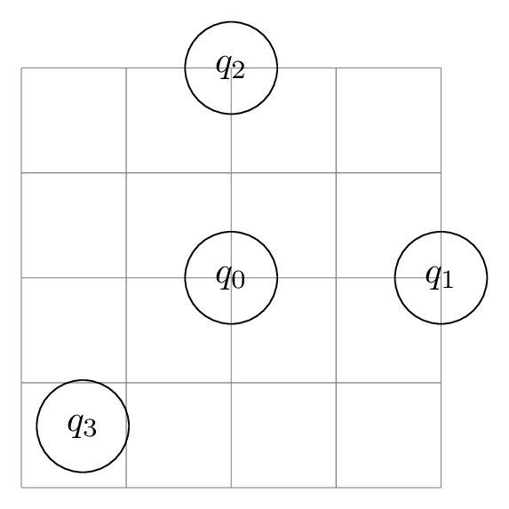
and here is the corresponding code:

3. Customize the initial state

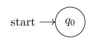
Now let's focus on state types. automata library gives us the option to easily create an initial state with the option initial (it should be used with state option.) This option will draw an arrow from 'start' text towards our node. The next code shows how to create an initial state.

a. How to Position and Change "start text" 

Usually after a few examples, we don't need to state the start text every time we draw another diagram. We can alter the text using initial text option. If we want it blank, we just need to type initial text = {}. Another option we have is the arrow length. We can set it by using initial distance command, it takes any distance as a parameter.

Example: The following code creates an initial state with initial text Start here, 1.5cm to the right far from the state.

b. Change initial state to diamond shape

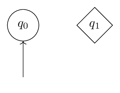
There is another kind of notation supported by automate library, which implies an initial state by drawing a diamond around it. Actually, initial option is by default set to initial by arrow, we can instead use initial by diamond. To use it we also need to add shapes library to our environment.

Example: In the following example, we initiated our state by approaching it from below with no text on the starting end, and with a longer arrow. After that, we drew another initial state with a diamond.

4. Customize the accepting state

Our next state type is an accepting state, which we can create by using accepting option, it will draw a double line border around our state. Following code implements an initial state.

a. Accepting state with an arrow out of the state

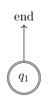
We can also show an accepting state by drawing an arrow coming out of the state. The keyword for this option is accepting by arrow and it works similarly to initial commands.

By default, the arrow will be pointing right. We can change it by using accepting below, accepting above or accepting left commands.

We can also add text to the end of the arrow by adding accepting text option. Lastly, we can change its length with accepting distance option.

Example: In the following example we drew an accepting state that ends with a 1 cm arrow towards above to an 'end' statement.

5. Create state with a split

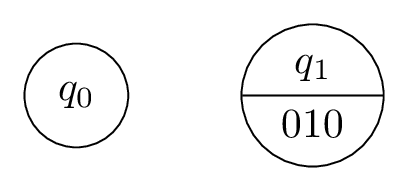
We have one more state option beside our regular state, a state that has an output. We can use it with state with output option, it creates a state split horizontally. Name of the state goes above and the output goes below.

We can write to the below part using \nodepart{lower} syntax in our content. Actually, the state option by default has been set to state without output and we can also use it to create a regular state. In the following example we created a state without output and a state with output side by side.

6. Connect states with transitions!

Now that we went over creating and formatting the states, let's turn our focus to transitions.

To draw the arrows, we can use \path command of TikZ with -> parameter (check the post Exploring TikZ arrows for more details). After that, we need to state each arrow line between states using edge command.

We also need to show how the input will be carried through our diagram. We can place our symbols inside nodes near the arrows using node command. We can place these symbols in a similar way to our states using above, below, left and right commands, or we can give auto option to tikzpicture to place them where it sees fit. Lastly, we need to use these commands between the names of the two connecting state.

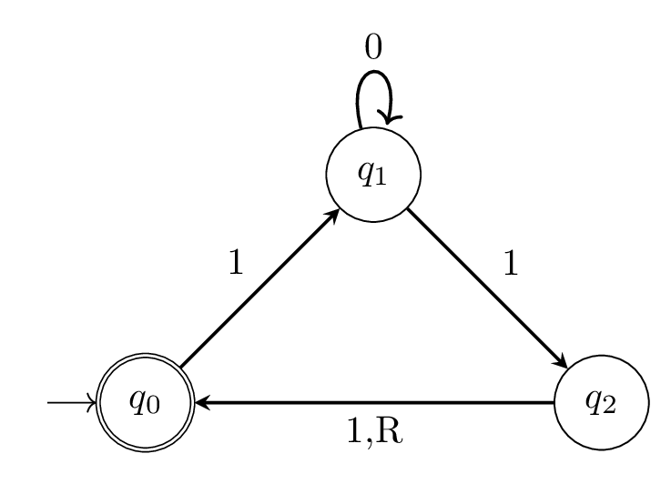
Example: The next code shows three states connected through labeled arrows: 

a. How to bend transition arrows? 

When we add more transitions, we need to take precautions to avoid overlapping arrows. We can use bend left and bend right commands to have curved arrows. To set the bending angle, we can give bend angle styling option with an angle parameter to the tikzpicture environment.

In the following code, we added three more transitions and bended our arrows to avoid collisions.

And here is the obtained automaton:

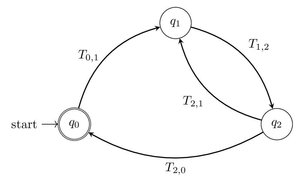
The auto option for labelling did the best it can, but there is room for enhancement. In this case, we can use the keywords left, right, above and below and also specify the label distance from the line using below=<value>. These changes will help get a cleaner look!

Change the global style of states and transitions

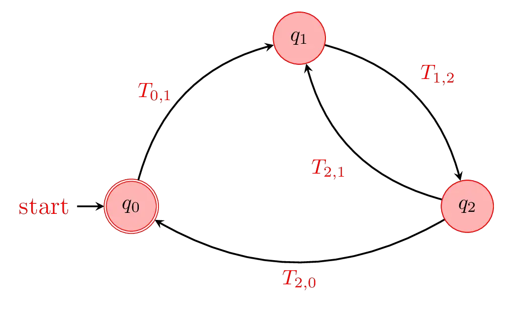
In some cases, we may want to emphasize different types of states with different colors, lines or fonts. We can style the states individually, but we also have the option to style every node we have on the environment.

We just need to add every state/.style option to our tikzpicture. If we don't want to change current options, we can use every state/.append style. We also have two more options for initial by arrow and accepting by arrow states, to alter the style of start/end texts and arrows. 

The next code changes all our states' line and filling colors to red, creates a bolder arrow and changes the size and color of the 'start' text.

Loop arrow orientation

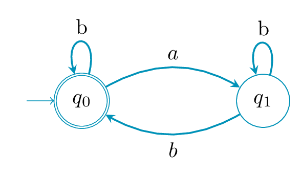
The following example highlights how one can change the direction of the loop arrow from right to left using the option every loop/.style{}. Here is the corresponding code:

and the obtained illustration:

For more details, check loops options in To path library of the PGF/TikZ manual.